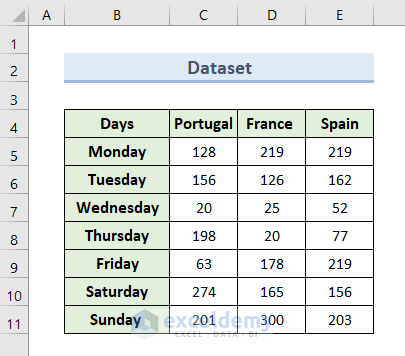
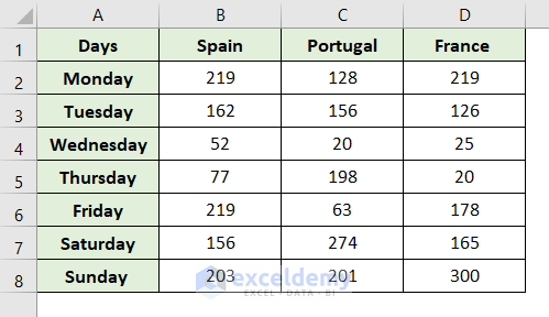
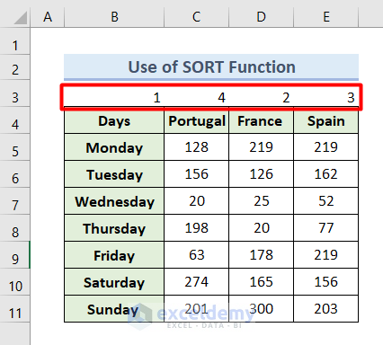
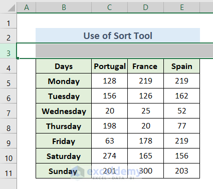
In this article,, we will demonstrate 3 easy methods to automatically rearrange columns in Excel using the following dataset comprising the amount of rain in a week in 3 countries in Europe.
Method 1 – Using Excel VBA
In the first method, we will use a simple VBA script to rearrange the columns automatically.
Steps:
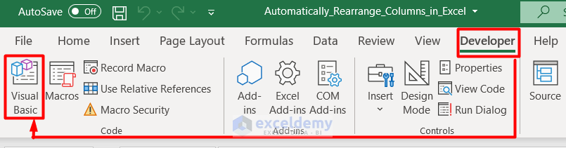
- Press F11 or go to the Developer tab and choose the Visual Basic icon (if the Developer tab is enabled).
A Visual Basic window will appear.
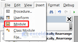
- Click on Insert and select Module.
- In the blank Module window that appears, input the following code:
Sub Rearrange_Columns()
Dim ColOrder As Variant, idx As Integer
Dim Fnd As Range, count As Integer
    ColOrder = Array("Days", "Spain", "Portugal", "France")
count = 1
Application.ScreenUpdating = False
   For idx = LBound(ColOrder) To UBound(ColOrder)
    Set Fnd = Rows("1:1").Find(ColOrder(idx), LookIn:=xlValues, LookAt:=xlWhole, SearchOrder:=xlByColumns, SearchDirection:=xlNext, MatchCase:=False)
    If Not Fnd Is Nothing Then
        If Fnd.Column <> count Then
            Fnd.EntireColumn.Cut
            Columns(count).Insert Shift:=xlToRight
            Application.CutCopyMode = False
        End If
    count = count + 1
    End If
Next idx
Application.ScreenUpdating = True
End Sub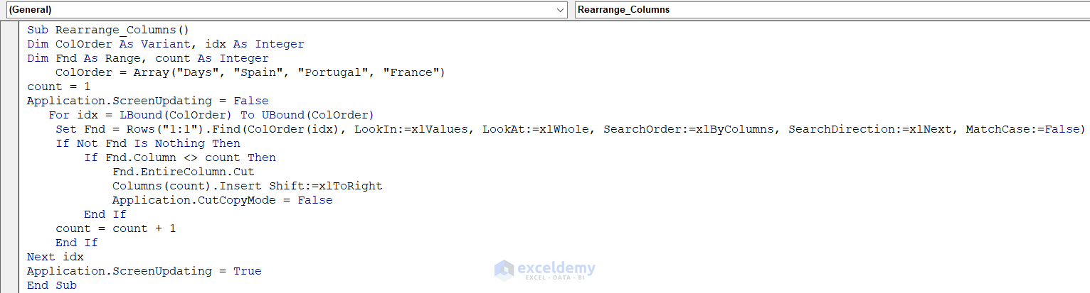
- Here, we change the parameters according to the way we want to rearrange the columns.
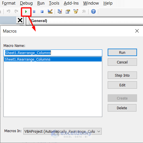
- Click on the RunSub button from the toolbar (or simply press the F5 key).
A Macros window will appear.
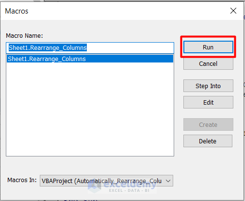
- Click Run to execute the VBA code.
The columns are rearranged following the parameters in the VBA code.
Method 2 – Using the SORT Function
To automatically rearrange columns while retaining the original order, we can use the SORT function. The SORT function helps to organize columns and can delete the old column after sorting.
The SORT function syntax is:
=SORT(array, sort_index, sort_order, by_column)Steps:
- Select the top row of the dataset. Or, insert a new row if it starts from row 1.
- In the new row, insert the numerical order in which you want to rearrange the columns like in the screenshot below.
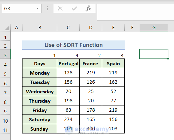
- Select the cell to place the new table, for example cell G3.
- Insert the following formula in cell G3:
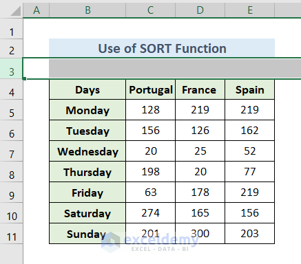
=SORT(B3:E11, 1, 1, TRUE)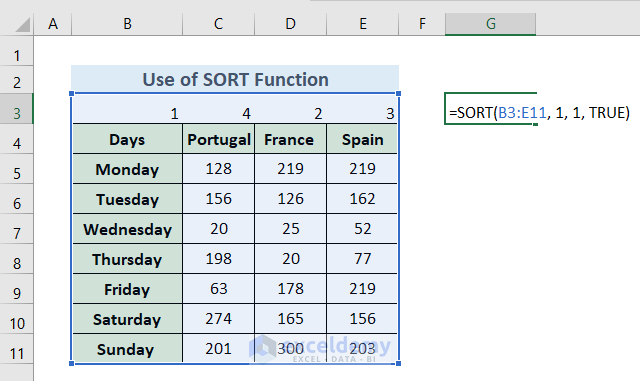
The array in the formula is set to the cell range (B3:G11) that we will sort. sort _index is set to 1 to indicate the 1st row of the selected dataset. sort_order is set to 1 for ascending order. The by_column perimeter is set to TRUE because we will sort columns, not rows.
- Press Enter.
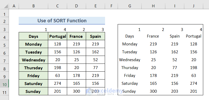
A whole new dataset is generated just beside the old one.
- Format the new table as desired.
The numerical order row can’t be deleted because it is a part of the formula. But it can be hidden.
- Simply right-click on the row and select Hide.
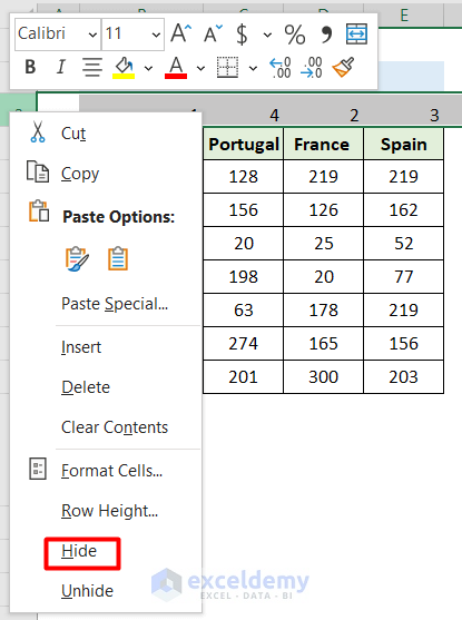
Following this process, you can rearrange the columns and hide the numerical order row.
Read More: How to Rearrange Columns in Excel
Method 3 – Using the Sort Tool
Steps:
- Select the top row of he dataset. Or, insert a new row if the dataset starts from row 1.
- As in the previous method, use this row to set out the new order of columns numerically.
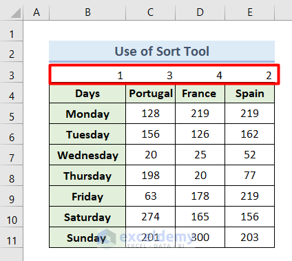
- Select the whole dataset.
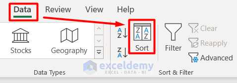
- Go to the Data tab and select the Sort tool from the Sort & Filter section.
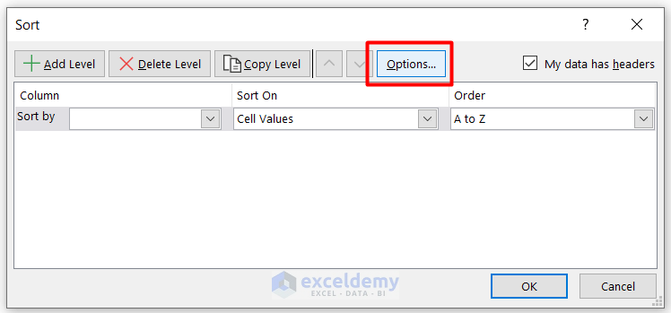
- In the Sort dialog box that appears, click Options.
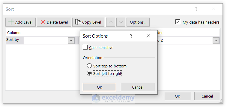
- From the Sort Options pop-up box, select the Sort left to right option and click OK.
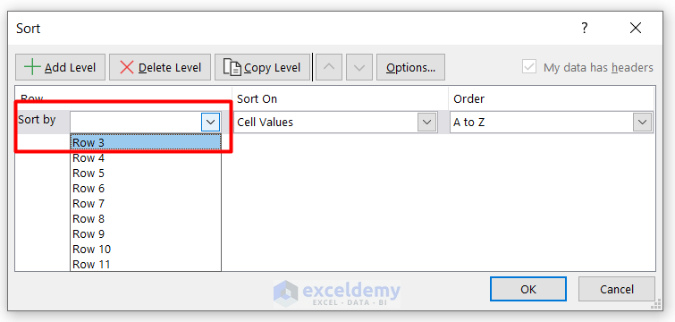
- In the Sort by section, select Row 3 (as we have started our dataset from Row 3) and then click OK.
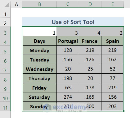
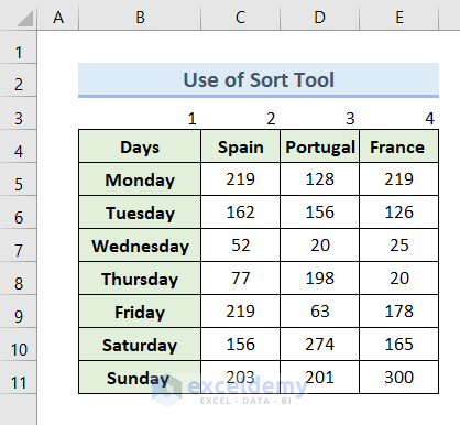
We have successfully reorganized columns with the Sort tool.
- Hide the numbers in the upper row of the dataset which we used to indicate column order.
Read More: How to Rearrange Columns Alphabetically in Excel
Things to Remember
- If there is any blank cell in the columns, you will be unable to rearrange them.
- In case of using VBA, make sure the columns start from column 1, because we are rearranging columns of the worksheet. Rows can be anywhere in the worksheet.
- It is good practice to keep a duplicate file of the original before rearranging.
Download Practice Workbook
Related Articles
<< Go Back to Rearranging in Excel | Data Analysis with Excel | Learn Excel
Get FREE Advanced Excel Exercises with Solutions!
