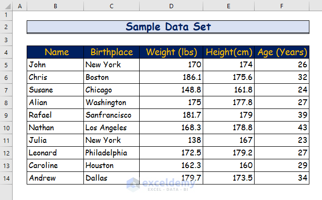
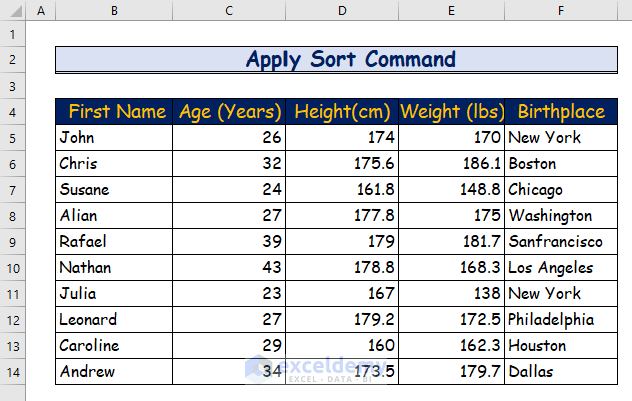
Dataset Overview
For the demonstration of rearranging columns in Excel, we will use the following dataset.
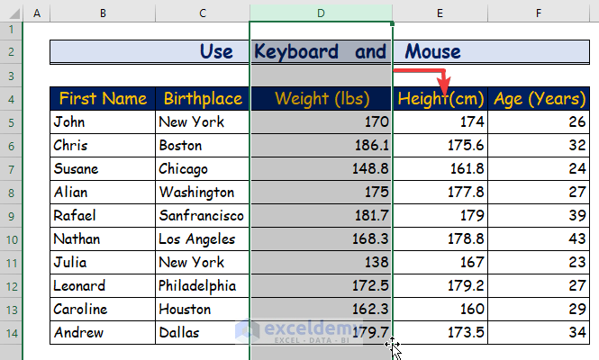
Method 1 – Using Keyboard and Mouse
Rearranging columns in Excel can be done easily using both the keyboard and mouse. Follow these steps to accomplish the task:
- Choose the column you want to rearrange.
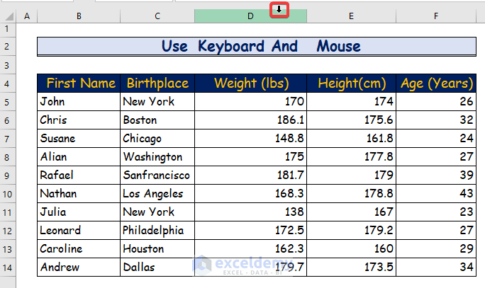
- Hover your mouse cursor over the top of that column.
- When the cursor changes into an arrow icon, click and highlight the entire column.
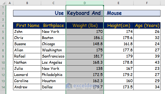
- Press and hold the Shift key on your keyboard.
- Position your mouse cursor on the highlighted column’s border (either to the left or right, as desired).
- Keep the cursor on the border until you see the cross-arrow pointer.
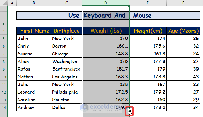
- Click and hold the left mouse button.
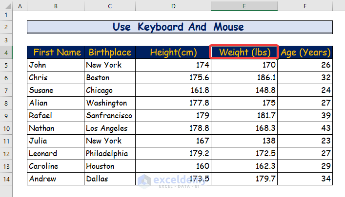
- Drag the column to its new position.
- Release the mouse button to drop the column where you need it.
- The column is now rearranged in its new place.
Read More: How to Automatically Rearrange Columns in Excel
Method 2 – Using the Cut and Paste Method
Moving columns in Excel is straightforward with the Cut and Paste method. Follow these steps to rearrange columns:
- Choose the column you want to move.
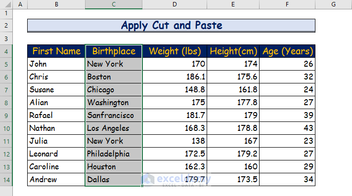
- Press Ctrl + X on your keyboard to activate Cut.
- You’ll notice a dotted border line around the selected column.
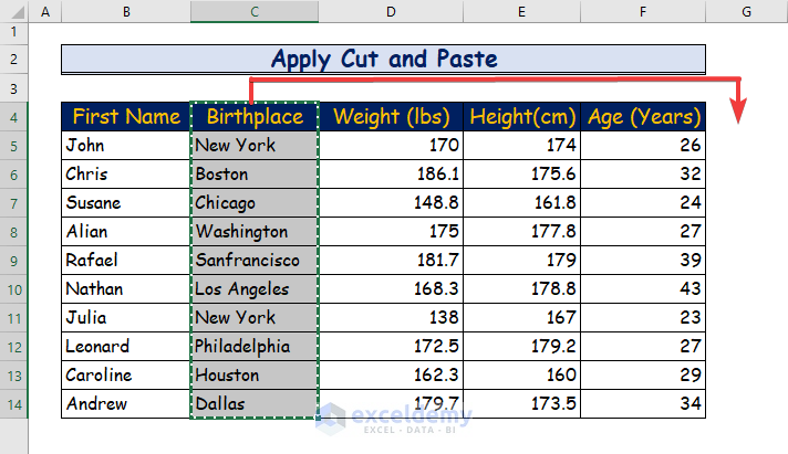
- Highlight a column to the right or left of where you want to paste the previously selected column.
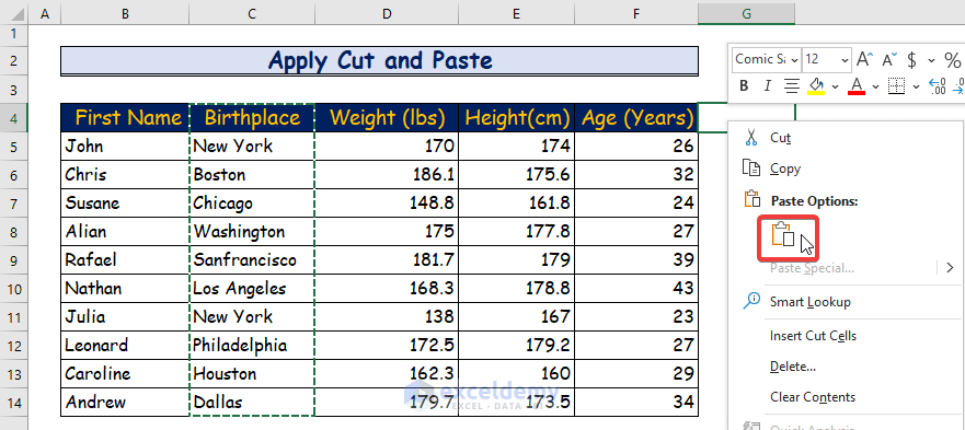
- Right-click your mouse and select the Paste.
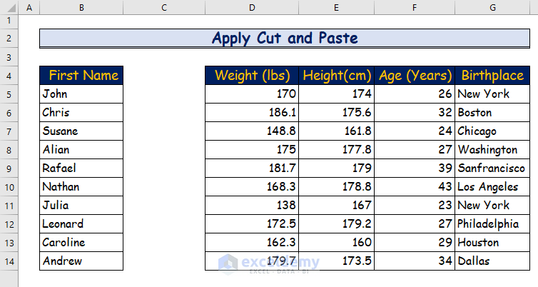
- The new column will appear in its rearranged destination.
Read More: How to Rearrange Columns Alphabetically in Excel
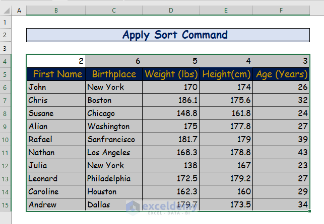
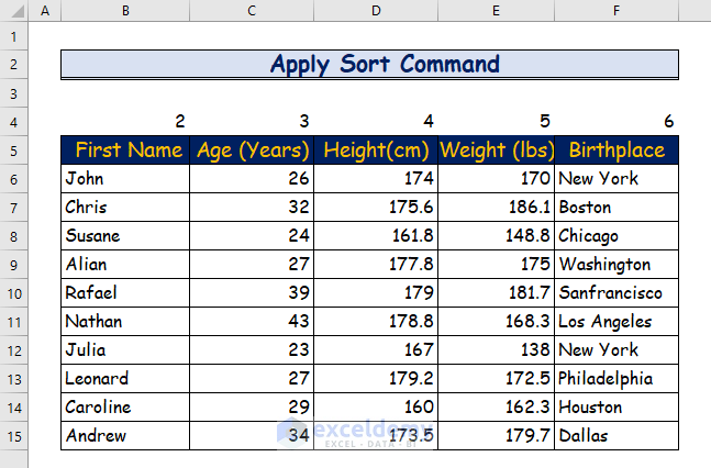
Method 3 – Using the Sort Command
If you need to rearrange columns in Excel, you can achieve this by applying the Sort command. Follow the steps below to move columns using this method:
- In your data set, add a new row at the very top.
- Right-click on the uppermost row of your data set and select Insert. This action will insert a new row.
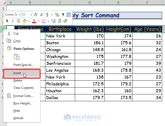
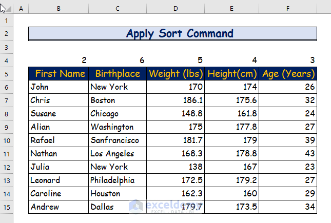
- Assign numbers to the new row based on your desired rearrangement order or requirement.
- Press Ctrl + A to select all of your data, including the new row.
- Go to the Data tab on the ribbon.
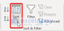
- Click on the Sort command in the Sort & Filter.
- A new dialog box will appear.
- Go to the Options menu and choose the Sort left to right
- From the Sort by drop-down list, select the number corresponding to the new row created earlier.
- Choose either Smallest to Largest or Largest to Smallest from the Order drop-down list.
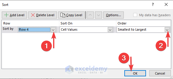
- The column will now be rearranged according to your specified order.
- If you added numbers to the table, you can delete them by right-clicking on the row number.
Read More: How to Rearrange Columns in Excel to Match Another Sheet
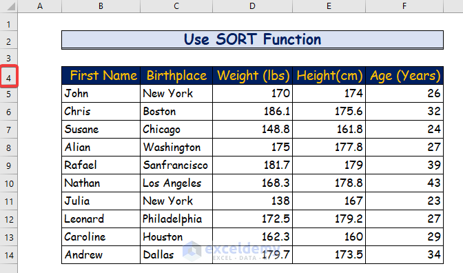
Method 4 – Using the SORT Function
Follow the steps below to use the SORT function:
- Add a new row at the top of your data table.
- Number the new row according to the rearrangement recommendation.
- Choose the cell where you want to rearrange your data table.
- In the formula bar, enter the following formula based on your data range.
- For example, if your data set spans from Cell B4 to F15, use the following SORT function:
=SORT(B4:F15,1,1,true)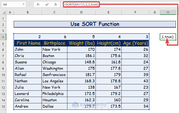
- Press Enter to apply the formula.
- Your data table will now be rearranged according to the specified order.
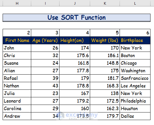
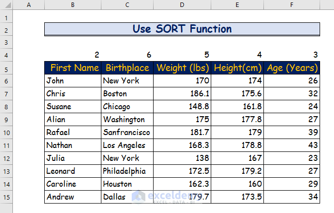
- You’ll notice the numbered row at the top of the data table.
- Unlike the previous method, you cannot delete this row because it’s part of the SORT function.
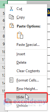
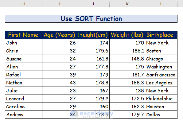
- Right-click on the row and choose the Hide option to conceal the entire numbered row.
Download Practice Workbook
You can download the practice workbook from here:
Related Articles
<< Go Back to Rearranging in Excel | Data Analysis with Excel | Learn Excel
Get FREE Advanced Excel Exercises with Solutions!
