Latest Posts From Raiyan Zaman Adrey

The "Refresh All" feature in Excel is essential for retrieving up-to-date data and sustaining correct analyses. However, at certain times this functionality ...

Method 1 - Excel SUMIF Greater Than Specific Value Select cell D20, apply the formula below, and press Enter. =SUMIF(C5:C17,">2") ...

What Is Slicer? An Excel slicer is a visual filtering tool that enhances data filtering. It is used in conjunction with tables, pivot tables, or pivot ...

In this article, we will demonstrate the use of Excel VBA to perform text to columns operations on fixed-width data types using the TextToColumns method. The ...
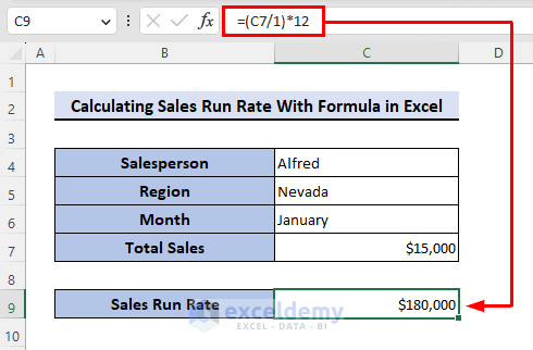
The sales run rate is used to estimate a company's potential future revenue based on its present revenue. It is determined by dividing the total current sales ...
See Our Reviews at


Dear Emely Phiri,
Thanks for reaching out to us. Let’s clear your confusion.
Think of it this way, you already know how one can calculate annual interest when one has the principle and the every month’s saving’s amount. If it is simple interest, you use the I=P*r*n formula and for compound interest, you use I=P*(1+r)^n-P.
Now, if I say, your principle is $1200, interest rate is 10% then the annual interest using the simple formula would be $1200*0.1*1=$120 right? Which means, the interest you are actually getting is $120/12=$10 every month. And if you save like $50 every month, the total amount in your account at the end of the first month and at the beginning of the second month will be $1200+$10+$50=$1260, where $1200 is your principle, $10 is the first month’s interest and $50 is the amount you further deposited into your account.
Now, as you have deposited $50 more, would the interest at the end of the second month and at the beginning of the third month be the same? Of course not.
At the beginning of the second month, the net amount in your account is $1260 right? Then, as the interest rate is 10%, so in that sense the annual interest using this new amount should be $1260*0.1*1=$126. So basically, the monthly interest this time becomes $126/12=$10.5. That means, at the end of the second month and at the beginning of the third month, the net amount in your account now is $1260+$10.5+$50=$1320.5, where $1260 is the net amount at the beginning of the second month, $10.5 is the monthly interest and $50 is the amount you save every month. And the same procedure goes on for the rest of the months as you are depositing money every month into your account.
For monthly compound interest, the procedure is mentioned in this article.
Hope, this clears your confusion. Have a great day.
Dear COLYNN BURRELL,
Thanks for reading our article. Try the following formula to resolve your issue.
=IF(C5="Fail", TEXT("Replace, Review", "[$-409]@"), "")The formula indicates that if cell C5 contains text Fail, then the formula will return Replace, Review. If not, then the result it will return will be blank.
Formula Breakdown
● TEXT(“Replace, Review”, “[$-409]@”)
This formula returns Replace, Review each time.
● IF(C5=”Fail”, TEXT(“Replace, Review”, “[$-409]@”), “”)
This formula returns Replace, Review only for the text string Fail.
Now to add red color to the output, use the conditional formatting feature as illustrated in this article.
● Select the range D5:D9.
● Go through these steps: Home >> Conditional Formatting >> New Rule.
● Now, select Format only cells that contain from the Select a Rule Type section.
● Select Specific Text.
● Type Replace, Review.
● Click on Format.
● Select Font.
● Click on the arrow down icon in the color section.
● Select the color red.
● Click on OK.
● Click on OK again.
● And the output will be as follows as you have desired.
Note: However, you can’t change the color of the output just after applying the formula. You have to use conditional formatting for that.
If the problem still appears, kindly send us your Excel file and specify the exact problem you are facing.
Thank you
Best Wishes,
Raiyan Zaman Adrey
Dear MARK GROENING,
Thank you for reading our articles. You wanted a formula to delete any random number and leave only text.
You can follow method 3 and method 5 of this article for your problem. The formulas mentioned here should work with your problem.
Using formula of method 3:
=TEXTJOIN(“”, TRUE,IFERROR(MID(B5, SEQUENCE(LEN(B5)), 1) *1, “”))
Using formula of method 5:
=SUM(MID(0&B5,LARGE(INDEX(ISNUMBER(–MID(B5,ROW($1:$99),1))*ROW($1:$99),),ROW($1:$99))+1, 1)*10^ROW($1:$99)/10)
Hope, this worked for your problem.
Regards,
Raiyan Zaman Adrey