How to Find Y Intercept in Excel (3 Effective Methods)

This tutorial will demonstrate how to find the y-intercept in Excel. When we are dealing with mathematical graphs, we often determine interception. The y interception represents the value of constant value c. By that, one can easily understand the main formula, y=mx+c. It shows how the values are creating the overall graph and moreover, it gives us the hint if the graph is going upward or downward. We can use this method to create graphs in the marketing sector or finance sector also. It can show us the pathway to make decisions. So, it is very important to learn how to find the y-intercept in Excel.

How to Find Y Intercept in Excel: 3 Effective Methods

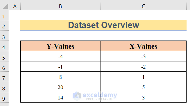
We’ll use a sample dataset overview as an example in Excel to understand easily. For instance, we have Y-values in Column B and X-values in Column C. The values are actually obtained from a straight-line equation. If you follow the steps correctly, you should learn how to find the y-intercept in Excel on your own. The steps are

1. Using Excel INTERCEPT Function to Find Y Intercept

In this case, our goal is to learn how to find the y-intercept in Excel by using the INTERCEPT Function in Excel. The INTERCEPT Function mainly deals with the x and y values of Excel and shows us the final y-axis interception. To learn this method we should follow the below description.

Steps:

First, insert the following formula in cell C11.

=INTERCEPT(B5:B9,C5:C9)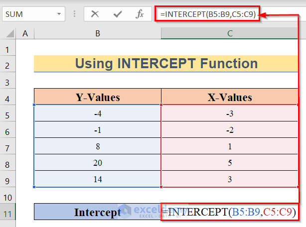

Next, press the Enter button.
Finally, you will get the y-intercept with the INTERCEPT function in Excel like the following image.

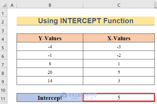
Thus, we can find the y-intercept in Excel by using the INTERCEPTION Function.

2. Use of Excel AVERAGE Function to Find Y Intercept

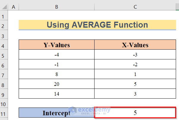
Now, we aim to learn how to find the y-intercept in Excel by using the AVERAGE Function. The AVERAGE function is mainly useful when needing to find the mathematical means or use mathematical means in some cases. We can easily do this by following the below steps.

Steps:

To begin with, we used a similar dataset to the first method and insert the following formula in cell C11.

=AVERAGE(B5:B9)-SLOPE(B5:B9,C5:C9)*AVERAGE(C5:C9)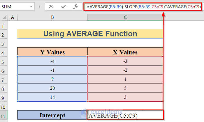

🔎 How Does the Formula Work?

AVERAGE(B5:B9): In the first portion, we have used the AVERAGE function and in the function, we have taken the input from B5 to B9 The function will take the values from these cells and give us the average value accordingly.
SLOPE(B5:B9, C5:C9): From this section, we will get an idea about the SLOPE function. The function takes the input in two sections. In the first section, we have inserted B5 to B9 cells which represent y-values and in the second portion, we have inserted C5 to C9 cells which represent x-values.
AVERAGE(B5:B9)-SLOPE(B5:B9, C5:C9)*AVERAGE(C5:C9): This is the whole equation. At first, we have taken the average of cells B5 to B9. Then, used the SLOPE function from C5 to C9 cells and multiplied the result by the average of cells C5 to c9 Thus, your y-intercept function is ready.

In addition, hit the Enter button.
Finally, you will get the y-intercept with the AVERAGE function in Excel like the following image.

Hence, we have learned how to find the y-intercept in Excel by using the AVERAGE Function.

3. Finding Y Intercept by Using Chart

In this case, our goal is to learn how to find the y-intercept in Excel by using the Chart in Excel. The Chart mainly deals with the x and y values of Excel and shows us the final x and y axes values and by that, we can easily determine the y-intercept in Excel. To learn this method we should follow the below result.

Steps:

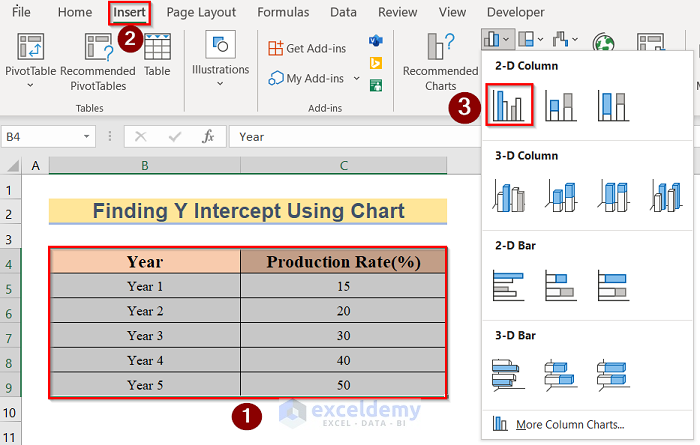
First, we arranged a dataset. For instance, we have Year in Column B and Production Rate(%) in column C.

Next, go to Insert >> Insert Column or Bar Chart option> 2-D column options.

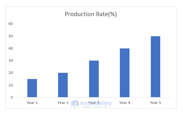
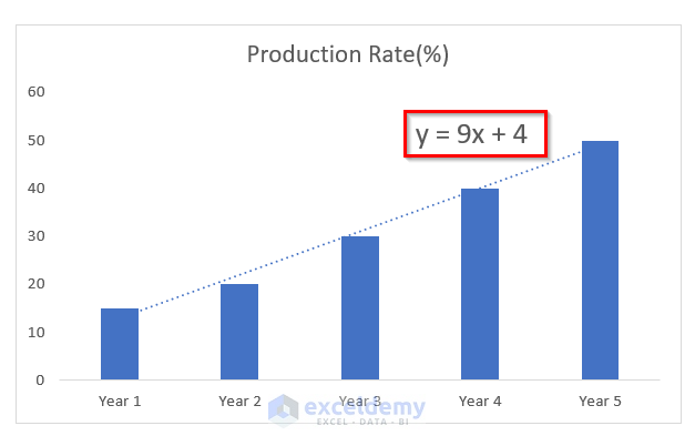
Subsequently, you will get the column chart like the below image. For this case, we have inserted the Production Rate(%) in the y-axis and the Year in the x-axis.

Furthermore, go to Chart Elements>Trendlines>More Options.

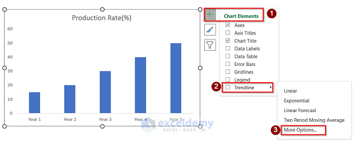
Afterward, in the Format Trendline window, go to Trendlines Options>select Display Equation on Chart options.

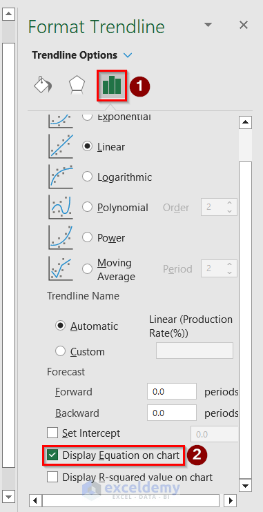
Finally, we have got the linear equation for this chart, y=9x+4. If we compare the linear equation with the y=mx+c equation, then we will get the result c=4. Actually, the value of constant (c) represents the y-intersection value for this chart. So here, the y-intercept of this data is 4.

Thus, we have learned to find the y-intercept in Excel by using the Chart in Excel.

How to Find SLOPE in Excel

In this section, we aim to learn how to find slopes in Excel by using the SLOPE Function. The SLOPE function mainly takes in the y and x values and then gives away the required slope of the line. We can find the slope in Excel by following the below steps.

Steps:

First, we used a similar dataset to the first method and insert the following formula in cell C11.

=SLOPE(B5:B9,C5:C9)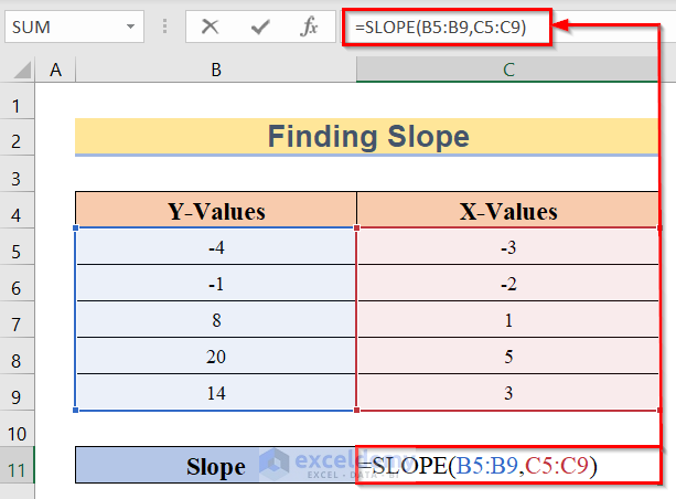

Second, click on the Enter button.
Last, you will get the slope with the SLOPE function in Excel like the following image.

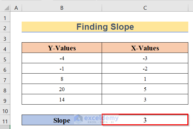
Therefore, we have managed to show how to find slopes in Excel by using the SLOPE Function.

Things to Remember

The most important thing about using the INTERCEPT or SLOPE function is you have to insert the y-values and then insert a comma and afterward insert the x-values. It is extremely essential to follow this sequence. Otherwise, you won’t get the proper result accordingly.
In the case of using the functions, we must focus on the conditions properly. If the condition isn’t written properly then the desired result won’t be found.
We suggest you download the excel file and see it while using the formulas for better understanding.

Download Practice Workbook

You can download the practice workbook from here.

Finding Y-INTERCEPT.xlsx

Conclusion

Henceforth, follow the above-described methods. These methods will help you to learn how to find the y-intercept in Excel. We will be glad to know if you can execute the task in any other way. Please feel free to add comments, suggestions, or questions in the section below if you have any confusion or face any problems. We will try our best to solve the problem or work with your suggestions.