Example 1 – Start with an Initial Investment and No Recurring Deposits
You have some investible money, and you want to invest the money with the following details:
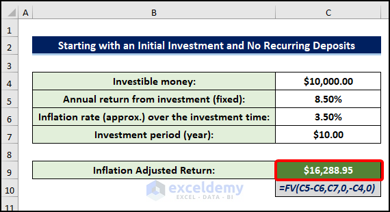
- Investible money: $10,000
- Annual return from investment (fixed): 8.5% per year
- Inflation rate (approx.) over the investment time: 3.5%
- Investment period: 10 years
What will be your inflation-adjusted return?
Steps:
- Input the information in the cell range C4:C7.
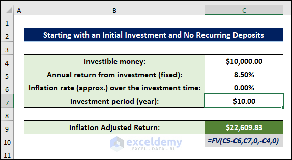
- This is the return you will get (following image). Use the FV formula with the arguments from the cells you input.
- In real life, you will get actually a return of the amount of $22,609.83 with the following formula (inflation is zero):
- The purchasing power of your value will be $16,288.95.
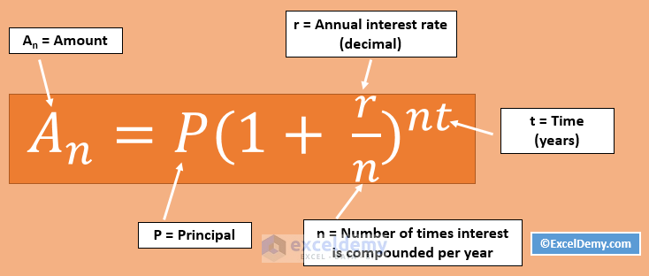
- You will also come out with the same value if you use the following universal formula. For the value of r, use the real rate of return (real rate of return = annual return – inflation rate).
Read More: How to Apply Future Value of an Annuity Formula in Excel
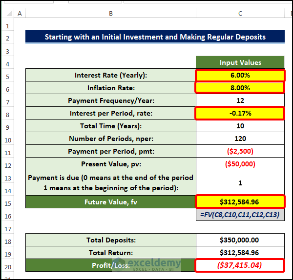
Example 2 – Start with an Initial Investment and Make Regular Deposits
Because of the deposits, the future value calculation will need to be adjusted.
In this example, we’re showing a scenario with the following details:
- Your initial investment: $50,000
- You’re paying a regular monthly deposit: $2500
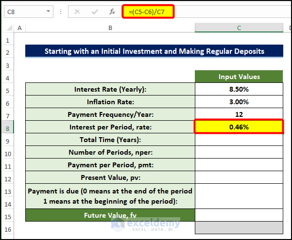
- Interest rate (yearly): 8.5%
- Inflation rate (yearly): 3%
- Payment Frequency/Year: 12
- Total Time (Years): 10
- Payment per Period, pmt: $2,500.00
- Present Value, PV: 50000
- Payment is done at the beginning of the period
Steps:
- Calculate the investment per period. Select cell C7 and enter the following formula:
=(C5-C6)/C7- In cell C7, we have calculated the Interest per Period by subtracting the Yearly Inflation Rate from the Yearly Interest Rate and then dividing the value by the Number of Payments per Year.
- The following image shows the output.
- Enter the total time period of depositing money in cell C9.
- Select cell C10 and enter the following formula:
=C9*C7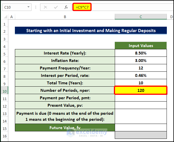
- Put the Payment per period that you are going to use in the cell C11.
- Input the present value of the money or one-time deposit in cell C12.
- Enter 1 in cell C13. This denotes the payment due at the beginning of the payment period.
- Enter the following formula in cell C15.
=FV(C8,C10,C11,C12,C13)
- Select cell C18 and enter the following formula:
=-C12+(-C11)*C10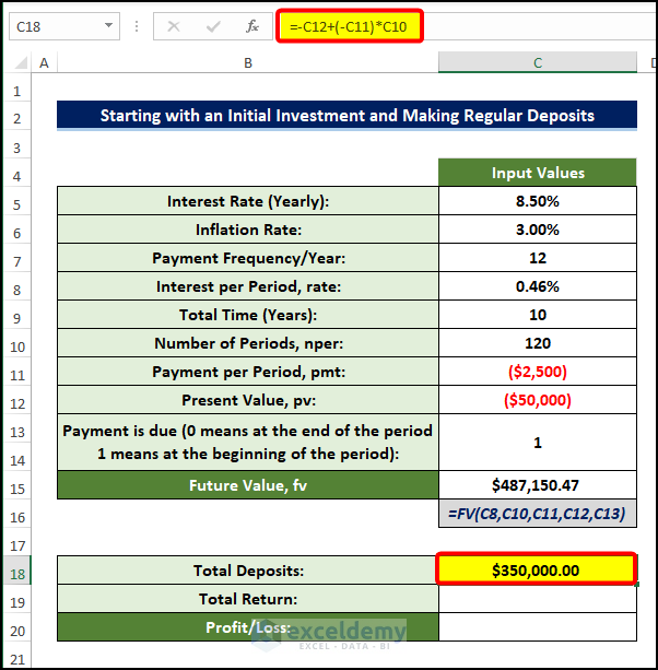
- Choose cell C19 and enter the following formula:
=C15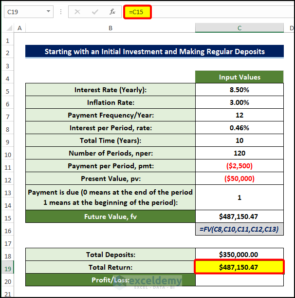
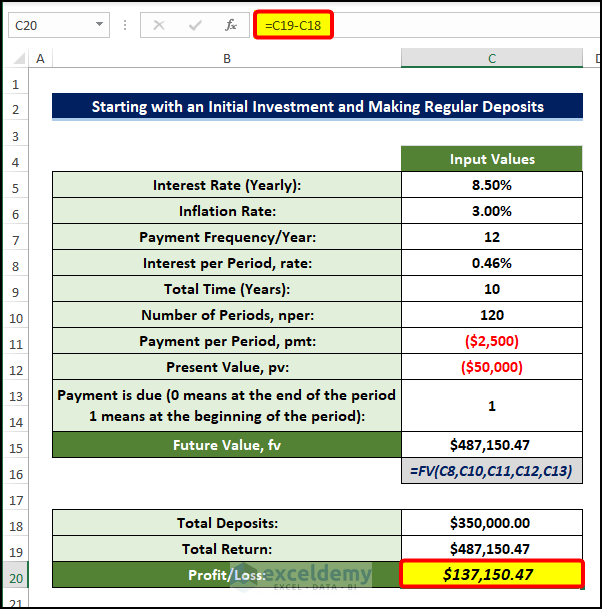
- Insert the following formula in cell C20:
=C19-C18- You’ll get the Future value of the deposit made over the course of the payment period.
- In cell C7, we have calculated the Interest per Period by subtracting the Yearly Inflation Rate from the Yearly Interest Rate and then dividing the value by the Number of Payments per Year.
- If the Yearly Return is lower than the Inflation Rate, you will effectively lose money. Consider the example on the screenshot.
Read More: How to Calculate Future Value of Growing Annuity in Excel
Download Practice Workbook
Download this practice workbook below.
Related Articles
- How to Apply Present Value of Annuity Formula in Excel
- How to Calculate Present Value of Uneven Cash Flows in Excel
- How to Calculate Future Value of Uneven Cash Flows in Excel
- How to Calculate Present Value of Future Cash Flows in Excel
- How to Calculate Future Value in Excel with Different Payments
- How to Calculate Present Value of Lump Sum in Excel
- How to Make a Time Value of Money Calculator in Excel
- How to Calculate Present Value in Excel with Different Payments
- Calculate NPV for Monthly Cash Flows with Formula in Excel
<< Go Back to Time Value Of Money In Excel | Excel for Finance | Learn Excel
Get FREE Advanced Excel Exercises with Solutions!

Hi, I like your website it is very easy to understand (for a simple mind like mine).
There is one example that nobody seems to show (I have been surfing to web for a while trying to find a solution to this problem), may be you might be able to help me please.
Here is the problem as an example;
1. I receive net $2000 p.m. from rent.
2. I invest this in an investment account that gives me 10% interest p.a.
3. Every year the rental is increase of 2.5% per year
4. Using excel FV calc., FV=(rate=2.083%,nper=120,PMT=?,PV=0,1)
5. The PMT has to be indexed somehow to take into consideration the 2.5% increase in yearly deposits in-line with inflation.
6. I know the answer at the end should be $453,624.65 (I printed something off a while back but I’ve lost the website) but I cannot come anywhere near this figure.
So, the question is how do I configure this FV formula?
If you can help me, I would be extremely grateful. Thank you in advance.
if i deposit 1000 each year to a pension bank for 41 years with an inflation of 1.40% and an interest of 4.40%, then how am i able to get the answer in one FV formula. I’ve already made a table for each year but am unable to get the answer in one formula.
Hi, ADRIAAN!
Thank you for your query.
The FV formula that you need for your solution will be like this:
=FV([(Interest Rate-Inflation Rate)/Frequency of Payment Per Year],[Frequency of Payment Per Year * Total Years],[-Payment Per Period], Present Value,0)So, with your given values, the formula would be:
=FV(3%,41,-1000,0,0)Regards,
Tanjim Reza
if i deposit 1000 each year to a pension bank for 41 years with an inflation of 1.40% and an interest of 4.40%, then how am i able to get the answer in one FV formula. I’ve already made a table for each year but am unable to get the answer in one formula.
Hi, A!
Thank you for your query.
The FV formula that you need for your solution will be like this:
=FV([(Interest Rate-Inflation Rate)/Frequency of Payment Per Year],[Frequency of Payment Per Year * Total Years],[-Payment Per Period], Present Value,0)So, with your given values, the formula would be:
=FV(3%,41,-1000,0,0)Regards,
Tanjim Reza
Hi, thank you for this information
How can you incorporate ‘fees’ (such as pension fund fees e.g per annum fee of 0.7%) into the rate function?
Thanks,
Jack
Hi Jack
Thank you for your query.
It would be very kind of you if explain your problem in detail. Perhaps, you can send us your problem at [email protected] to get better assistance.
From your query, it seems like you want to calculate in Excel using the RATE function and insert a certain fee as a percentage in the function.
The RATE function returns the interest rate per period of an annuity. The syntax of the RATE function is as follows.
RATE(nper, pmt, pv, [fv], [type], [guess])
Where,
● Nper: Required. The total number of payment periods in an annuity.
● Pmt: Required. The payment made each period and cannot change over the life of the annuity. Typically, pmt includes principal and interest but no other fees or taxes. If pmt is omitted, you must include the fv argument.
● Pv: Required. The present value — the total amount that a series of future payments is worth now.
● Fv: Optional. The future value, or a cash balance you want to attain after the last payment is made. If fv is omitted, it is assumed to be 0 (the future value of a loan, for example, is 0). If fv is omitted, you must include the pmt argument.
● Type: Optional. The number 0 or 1 and indicates when payments are due.
● Guess: Optional.
As you can see, you cannot directly incorporate any fee as a percentage in the RATE function. However, you can indirectly use a percentage in a formula that has the RATE function.
I am going to discuss 2 such examples.
Example 1:
Let’s assume that you have borrowed $8000 for 4 years. The monthly payment is $200. Now, if you use the RATE function here, you will get a 9.24% annual loan rate. But in practice, you may need to adjust your loan. So in that case, you can incorporate a percentage.
The formula in C8 is
=RATE(C3*12, (-1)*C4, C5)*12-C7In the image above, we have subtracted a percentage (0.07%, our adjusting factor in C7) from the annual rate of the loan. In a similar fashion, you can manipulate your dataset the way you want.
Example 2:
Suppose you got a loan of 20% on the value of your certain asset. Now, you can incorporate this 20% in the RATE function. The formula in C7 is
=RATE(C3*12, (-1)*C4, C5*20%)*12
Here, C5*20% represents the loan amount ($8000).
This is how you can incorporate any value indirectly in the RATE function. To learn more, have a look at this article.
How to Use RATE Function in Excel (3 Examples)