8 Ways to Remove Duplicates in Excel Without Losing Data

 

Managing duplicate records is crucial for accurate data analysis in Excel. Duplicate data in Excel can cause inaccurate calculations, bloat file sizes, and create confusion. Excel offers multiple ways to remove duplicates.

In this tutorial, we will show 8 ways to remove duplicates in Excel without losing data.

1. Remove Duplicates Tool

Excel’s built-in Remove Duplicates feature offers a quick solution with a user-friendly interface.

Steps:

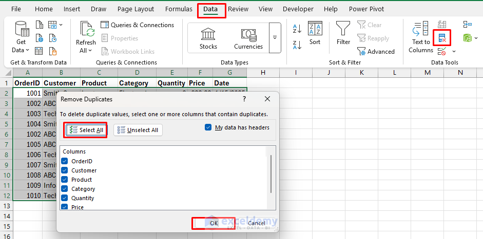
• Select your data range, including headers.
• Go to Data tab >> from Data Tools group >> select Remove Duplicates.
• Check/uncheck columns to determine which combinations create duplicates.
• Click OK.

Case:

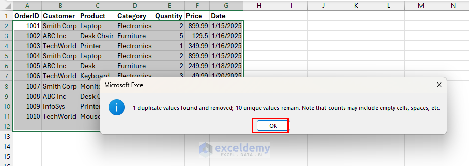
• If we select all columns, only row 6 (OrderID 1002) would be removed as it’s an exact duplicate of row 1.
• Excel will display a message that 1 duplicate value was found and removed.

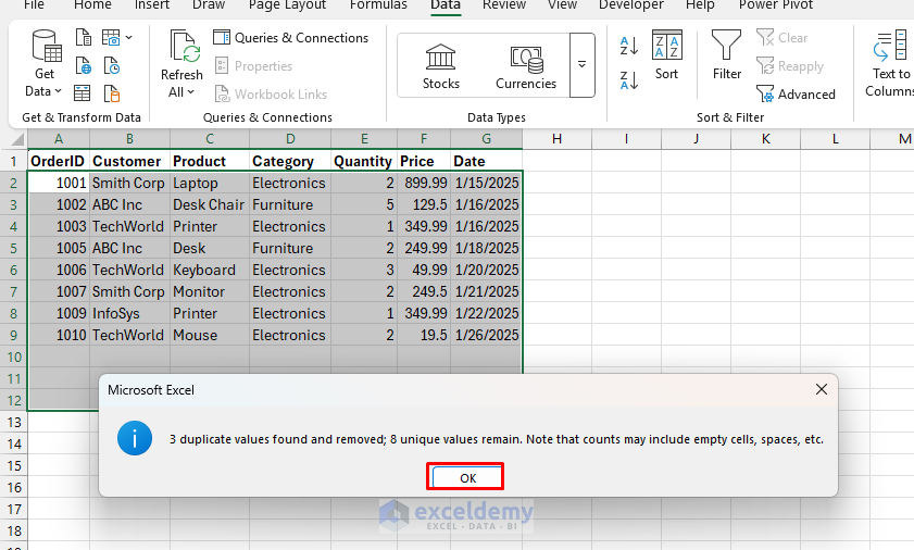
• If we uncheck OrderID and check all other columns.

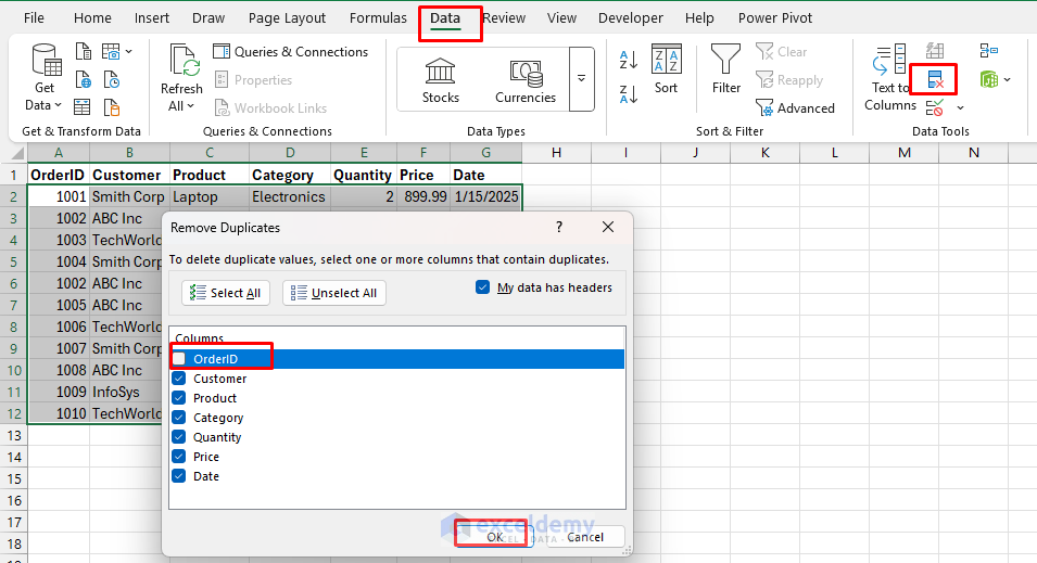
• Rows 5, 6 and 8 would be removed as duplicates.

Advantages:

• Simple to use with a visual interface.
• Works directly on your data.
• Can specify which columns to check.

Considerations:

• Permanently deletes duplicate rows.
• Keeps only the first instance of each record.
• Original data cannot be recovered unless you’ve made a backup.

Pro Tip: Always copy your data to another sheet before using this tool if you need to preserve the original dataset.

2. Advanced Filter (Unique Records Only)

Advanced Filter provides more control by letting you copy unique records to a new location.

Steps:

• Organize your data with headers.
• Go to Data tab >> from Sort & Filter group >> select Advanced.
• Select Copy to another location.
• Select your data range in List range: A1:G12.
• In Copy to: J1.
• Check Unique records only.
• Click OK.

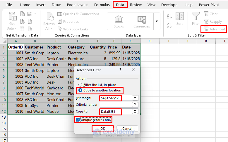
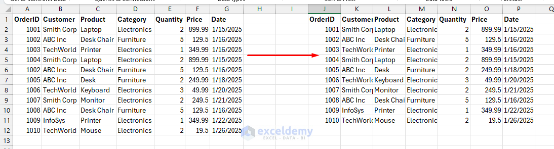
The duplicate row 6 (OrderID 1002) would be excluded from the results. Data will be copied to cell J1 and below, excluding the duplicate row.

Advanced Example: To identify transactions with duplicate product info regardless of OrderID, you could:

• Set up a criteria range with headers (B1:G1).
• Apply Advanced Filter with this criteria range to find identical transactions.

Advantages:

• Preserves original data.
• Copies only unique records to another location.
• Works with complex criteria if needed.

Considerations:

• Requires available space for the filtered results.
• Needs manual refresh when source data changes.

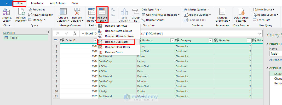
3. Power Query (Get & Transform)

Power Query offers a robust solution that preserves original data and can handle large datasets.

Steps:

• Select your data.
• Go to Data tab >> from Get & Transform Data group >> select From Table/Range.

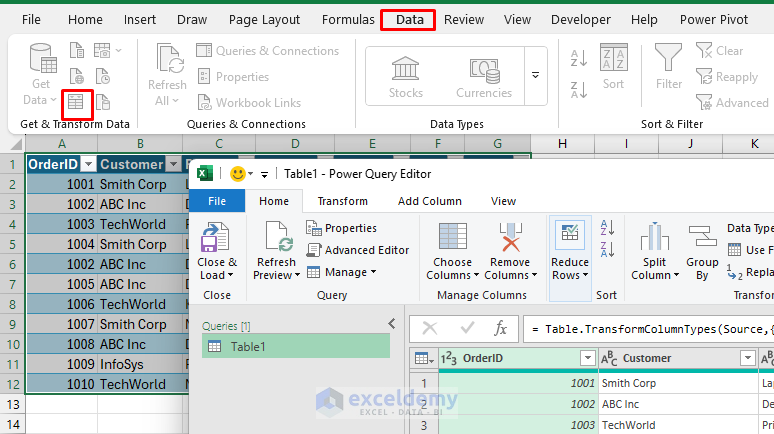
• Select columns for comparison (you can select all columns or only specific ones).
• Go to Home tab >> Remove Rows group >> Remove Duplicates.
• Click Close & Load to import results to a new sheet.

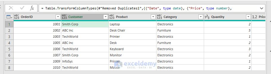
Example:

• If we remove duplicates based on all columns, only row 6 (OrderID 1002) would be removed.

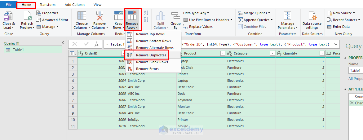
• If we remove duplicates based only on Customer, Product, Quantity, Price, and Date (excluding OrderID), both rows 4 and 8 would be identified as duplicates.

Output:

Advantages:

• Creates a separate result set that can be refreshed.
• Handles large datasets efficiently.
• Preserves original data.
• Can be part of a repeatable process.
• Advanced transformation capabilities.

Considerations:

• Requires a basic understanding of Power Query.
• Uses more resources for very large datasets.
• Additional steps are needed for complex deduplication logic.

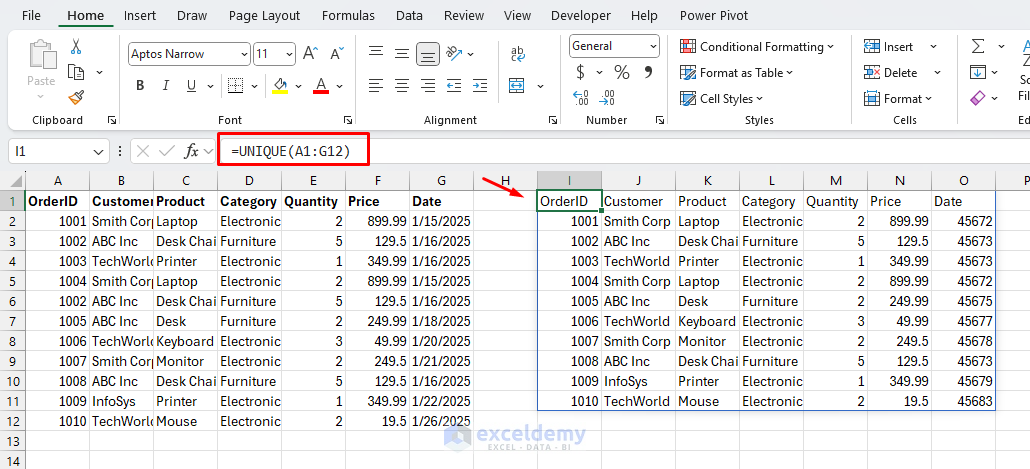
4. UNIQUE Function (Excel 365/2021)

For newer Excel versions, the UNIQUE function dynamically extracts distinct values.

Remove Duplicate Rows:

• Select cell I1 and insert the following formula.

Formula:

=UNIQUE(A2:G10)

You get a spill range with all unique rows. This list updates if you change the source data. This returns all unique rows from our dataset, excluding the duplicate row 6.

Unique Products by Category: To extract unique combinations of Product and Category.

• Select a cell and insert the following formula.

Formula:

=UNIQUE(C2:D10)

This formula will return a spill range with all unique product lists.

Unique Customer List: To get a list of unique customers.

• Select a cell and insert the following formula.

Formula:

=UNIQUE(B2:B10)

This formula will return a spill range with all unique customer names.

Advantages:

• Creates dynamic results that update automatically when source data changes.
• Non-destructive to source data.
• Can be combined with other functions.
• Returns unique combinations across multiple columns.

Considerations:

• Only available in Excel 365 and Excel 2021.
• Creates a spilled array formula (expands automatically).
• May require workspace planning.
• Cannot handle very complex deduplication logic.

5. Conditional Formatting + Filter

This visual approach helps to highlight and then filter duplicates.

Steps:

• Select your data range.
• Go to Home tab >> from Conditional Formatting >> select Highlight Cells Rules >> select Duplicate Values.

• Choose formatting style: Light Red Fill with Dark Red Text.
• Click OK.
• Excel highlights duplicate cells (by column).

• Go to the Data tab >> select Filter.
• Filter by cell color to show duplicate or unique values.
• For unique select Automatic for duplicate select Color.

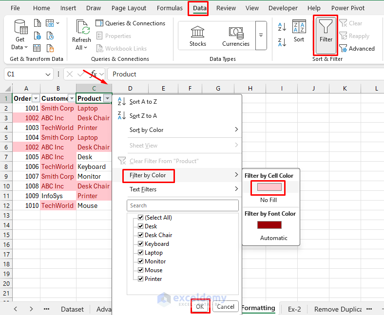
Unique:

Duplicate:

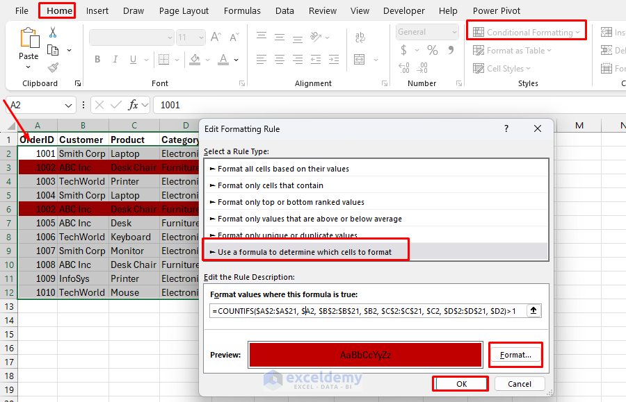
If you want to highlight entire duplicate rows, use a formula rule like:

• Go to Home tab >> from Conditional Formatting >> select >> New Rule.
• Select Use a formula to determine which cells to format.
• Insert the following formula:

=COUNTIFS($A$2:$A$12, $A2, $B$2:$B$12, $B2, $C$2:$C$12, $C2, $D$2:$D$12, $D2, $E$2:$E$12, $E2, $F$2:$F$12, $F2, $G$2:$G$12, $G2)>1

• Select fill color.
• Click OK.

Advantages:

• Visually identifies duplicates before removal.
• Preserves all data.
• Allows selective removal.
• Works in all Excel versions.
• Helps understand duplicate patterns.

Considerations:

• Multi-step process.
• Requires manual filtering.
• Not automatically updating.
• The filter needs to be reapplied if data changes.

6. Pivot Table Method

Pivot Tables naturally aggregate data, effectively removing duplicates in the process.

Steps:

• Select your data.
• Go to the Insert tab >> select PivotTable.
• Select the Existing Worksheet and location.
• Click OK.

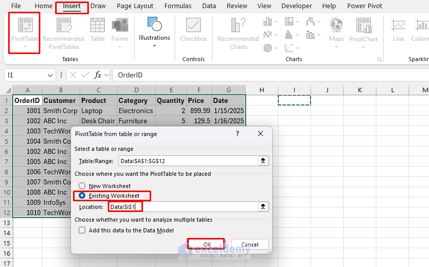
• From the PivotTable Fields List;
• Drag these fields to Rows:
  • Order ID, Customer, Product, Category, Date.
• Drag these fields to Values:
  • Quantity, Price.

The duplicate rows (3 and 6) have been combined, showing the sum of Quantity (5+5=10) and Price (129.5+129.5=259).

If you want to exclude OrderID to show duplicate products and customers:

• Remove OrderID from the Rows area first.
• The resulting pivot table will only show transactions where everything is similar except OrderID.

Advantages:

• Can summarize duplicate data instead of just removing it.
• Handles large datasets efficiently.
• Automatically aggregates numeric values.

Considerations:

• Requires a basic understanding of Pivot Tables.
• May need further formatting after extraction.
• Aggregates numeric values by default (may not be desired for some fields).

7. COUNTIF Helper Column

This method adds a column to identify the first occurrences of each record.

Steps:

• Add a helper column (column H) with the header “Duplicate Check”.
• Use a formula to identify unique rows.
• Filter for the appropriate values to see only unique records.

Identifying Complete Duplicates:

• Select cell H2, and enter this formula.

Formula:

=IF((COUNTIFS($A$2:$A$12, $A2, $B$2:$B$12, $B2, $C$2:$C$12, $C2, $D$2:$D$12, $D2, $E$2:$E$12, $E2, $F$2:$F$12, $F2, $G$2:$G$12, $G2))=1, "Unique","Duplicate")

This formula marks duplicates where the entire row is a duplicate.

Ignoring OrderID: To identify duplicates based on transaction details, regardless of OrderID:

=IF((COUNTIFS($B$2:$B$12, $B2, $C$2:$C$12, $C2, $D$2:$D$12, $D2, $E$2:$E$12, $E2, $F$2:$F$12, $F2, $G$2:$G$12, $G2))=1, "Unique","Duplicate")

This formula marks rows 2,3,5,6, and 10 as “Duplicate” since they duplicate the transaction details.

Advantages:

• Shows which records are duplicates and keeps the original data.
• Can be customized to complex conditions.
• Identifies which rows are duplicates.

Considerations:

• Requires an additional column.
• The formula can become complex for multiple columns.
• Needs to be adjusted if data changes.
• Must be copied down for new data.

8. Formula-Based Extraction (INDEX/MATCH or FILTER)

For advanced users, combinations of INDEX, MATCH, and other functions can extract unique values.

Use INDEX/MATCH (older Excel versions): To extract unique customer names for a separate location.

• Select a cell and insert the following formula.

Formula:

=IFERROR(INDEX($B$2:$B$12,MATCH(0,COUNTIF($I$1:I1,$B$2:$B$12),0)),"")

Use FILTER (Excel 365/2021): To extract unique records while keeping all columns.

• Select a cell and insert the following formula.

Formula:

=FILTER(A2:G12, MATCH(A2:A12&B2:B12&C2:C12&D2:D12&E2:E12&F2:F12&G2:G12, A2:A12&B2:B12&C2:C12&D2:D12&E2:E12&F2:F12&G2:G12, 0)=ROW(A2:A12)-ROW(A2)+1)

Advantages:

• Highly customizable.
• Works when other methods fail.
• Can incorporate complex logic.
• Non-destructive to source data.
• Dynamically updates with source data changes.

Considerations:

• Requires advanced Excel knowledge.
• More complex to implement and maintain.
• May require array formulas in older Excel versions.
• Can be resource-intensive for large datasets.

Conclusion

Removing duplicates in Excel doesn’t have to be risky or complicated. Whether you’re working with small reports or large datasets, Excel offers multiple safe and flexible methods to identify and eliminate duplicates. Based on your data type, you can use these 8 ways to remove duplicates in Excel without losing data. The best method depends on your Excel version, data size, and whether you prefer formulas or tools. Mastering these 8 techniques ensures you’re prepared for any duplicate-cleaning challenge. Always back up your data before removing duplicates, especially when using methods that modify your original dataset directly.