10 Excel Formulas for Power Users

Excel offers advanced and complex dynamic formulas that elevate productivity and precision in data analysis. These advanced formulas go beyond the basics, offering unparalleled flexibility and functionality for tackling complex tasks. In this article, we will list and explore Excel formulas for power users.

1. VLOOKUP for Data Lookups

VLOOKUP is one of the most useful and powerful functions that look up values from large datasets based on specific values. It reduced time-consuming searching tasks though more advanced functions came later yet the power of VLOOKUP is endless.

Formula:

=VLOOKUP(C2,C2:G11,5,FALSE)

This formula looks for the value in cell C2 within the first column of the range C2:G11. When it finds an exact match (as specified by FALSE), it returns the value from the 5th column of the range (G2:G11). If no exact match is found, it returns #N/A.

• Always use FALSE for the last argument to ensure an exact match.
• The lookup value must be in the leftmost column of your table array.
• This method works best when your data is organized in a table-like structure.

2. INDEX-MATCH for Dynamic Lookups

INDEX-MATCH is a dynamic lookup formula that works for advanced lookups. In some cases, it offers greater flexibility than VLOOKUP or HLOOKUP.

Formula:

=INDEX(G2:G11, MATCH("Tablet", C2:C11, 0))

This formula retrieves the value from the range G2:G11 that corresponds to the row where “Tablet” is found in the range C2:C11.

Usefulness:

• This formula can look up in any direction, unlike VLOOKUP.
• It can handle issues with column changes or data rearrangements.
• Handles large datasets when paired with dynamic ranges.

3. XLOOKUP for Dynamic Lookup Solution

The XLOOKUP function is a dynamic lookup function that replaces older lookup functions like VLOOKUP and HLOOKUP with advanced functionality and fewer limitations.

Formula:

=XLOOKUP("Tablet",C2:C11, G2:G11, "Not Found", 0, 1)

The formula searches for the value “Tablet” in the product range and returns the corresponding value from the profit range. If “Tablet” is not found, it displays “Not Found.” The 0 specifies an exact match, and the 1 indicates that the search should look for the next larger value if an exact match isn’t found.

Usefulness:

• It can search both vertically and horizontally.
• It offers support for exact and approximate matches.
• Its error-handling feature makes it robust for real-world scenarios.

4. SUMPRODUCT for Multi-Criteria Calculations

The SUMPRODUCT function is a versatile formula for conditional summations, weighted averages, and more, making it a favorite among analysts.

Formula:

=SUMPRODUCT((B2:B11="East")*(F2:F11>10000)*(F2:F11))

The formula calculates the total sales in the “East” region where sales exceed 10,000. These arrays are multiplied elementwise, where only rows that meet both conditions contribute to their sales values. Finally, SUMPRODUCT adds up these filtered sales, giving the desired result.

• It performs multi-condition calculations in a single formula.
• You won’t need to use any helper columns.
• It is ideal for calculating totals, averages, and weighted scores across datasets.

5. FILTER for Dynamic Data Extraction

FILTER formula dynamically extracts data based on criteria, perfect for creating automated reports and dashboards.

Formula:

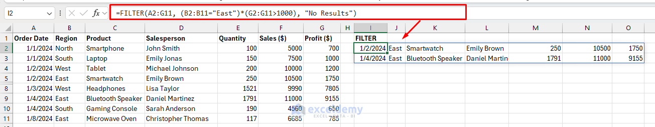
=FILTER(A2:G11, (B2:B11="East")*(G2:G11>1000), "No Results")

This formula filters rows where the region is “East” and profits exceed 1000. If no rows match both conditions, it returns “No Results”. This formula is useful for filtering data dynamically based on multiple criteria.

• B2:B11=”East”: The region is “East”.
• G2:G11>1000: The value in column G is greater than 1000.

Usefulness:

• Replaces manual filtering for more efficiency.
• Automatically updates results as the data changes.
• Excellent for creating interactive reports or dashboards.

6. LET for Enhanced Readability and Performance

The LET function can simplify complex formulas by storing intermediate calculations, improving performance and clarity.

Formula:

=LET(sales, 5000, profit, 700, profit/sales)

This formula calculates the profit margin (Profit ÷ Sales) for the “Smartphone” which simplifies calculations by defining variables directly within the formula.

• sales is defined as 5000.
• profit is defined as 700.

This approach is useful to improve readability and reusability in complex formulas by eliminating repetitive references.

Usefulness:

• It can reduce redundant calculations, improving speed.
• It makes complex formulas easier to understand.
• In dashboards and reporting, the LET function is useful.

7. LAMBDA to Create Reusable Functions

LAMBDA lets you create reusable custom functions directly in Excel, eliminating the need for VBA.

Formula:

=LAMBDA(sales,profit, profit/sales)(F2, G2)

This formula creates a reusable custom function that calculates the profit margin by dividing profit by sales. The LAMBDA function takes sales and profit as input, and the part (F2, G2) passes the values from cells F2 (sales) and G2 (profit) into the function, returning the profit margin for that specific row.

Usefulness:

• LAMBDA function defines names and creates reusable custom formulas.
• Encourages modularity and efficiency in large projects.
• Ideal for power users creating custom logic for repetitive tasks.

8. TEXTJOIN for Concatenating Data

TEXTJOIN can join text values from ranges into a single cell with a specific delimiter.

Formula:

=TEXTJOIN(", ", TRUE, C2:C11)

This formula joins the salesperson’s name with a comma delimiter from the specified range.

Usefulness:

• It handles concatenation for ranges with blanks seamlessly.
• Perfect for creating summaries or labels.
• Reduces the complexity of handling text data.

9. OFFSET for Dynamic Ranges

OFFSET creates dynamic references that adjust based on specific criteria, ideal for advanced reporting and analysis.

Formula:

=SUM(OFFSET(F11, -2, 0, 3, 1))

This formula calculates the sum of a range created dynamically using OFFSET. OFFSET starts from F11, moves up 2 rows (to F9), stays in the same column, and creates a range of 3 rows tall and 1 column wide (F9:F11). Then add the values in this range.

Usefulness:

• It enables dynamic data selection for calculations.
• Useful for rolling averages or moving window analysis.
• Works well with data validation and interactive dashboards.

10. AGGREGATE for Error Handling Calculations

AGGREGATE performs calculations while ignoring errors and hidden rows, making it robust for messy datasets.

Formula:

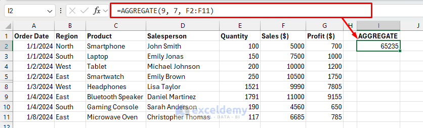
=AGGREGATE(9, 7, F2:F11)

This formula calculates the sum of the range F2:F11, ignoring the hidden rows that are rows 6 & 7.

• 9: It represents the SUM function.
• 7: It is the options parameter, which tells the formula to ignore hidden rows and errors.

Usefulness:

• Handles errors, and hidden rows without requiring helper columns.
• It supports a wide range of operations like SUM, AVERAGE, and MIN.
• Ideal for data cleaning and advanced analysis.

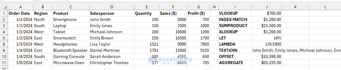
Output:

Bonus Tips for Power Users

• Dynamic Arrays: Use dynamic array functions like UNIQUE and SORT to build dynamic dashboards.
• Named Ranges: Pair formulas with named ranges for better readability and maintenance.
• Combine Formulas: Stack functions like FILTER and SEQUENCE to create intelligent, automated solutions.
• Error Handling: Functions like IFERROR, ISERROR, and IFNA functions help manage potential calculation errors by providing a fallback value.

Conclusion

These formulas are essential to handle large datasets and data analysis. These formulas can help power users to streamline workflows, handle complex scenarios, automate analysis, and generate dynamic reports. Explore these formulas’ dynamic and advanced functionalities. Mastering these advanced formulas will elevate your efficiency, precision, and creativity in Excel.