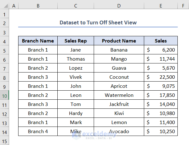
The sample dataset: Dataset to Turn Off Sheet View, showcases Branch Name, Sales Rep, Product Name, and Sales.
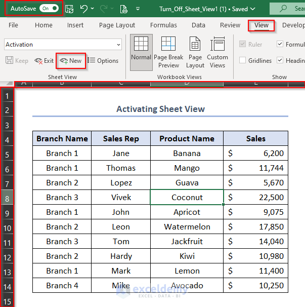
Step 1 – Activating Sheet View
The dataset is activated:
- AutoSave is turned On.
- The New option is available in Sheet View in View.
- Columns and Rows are marked black.
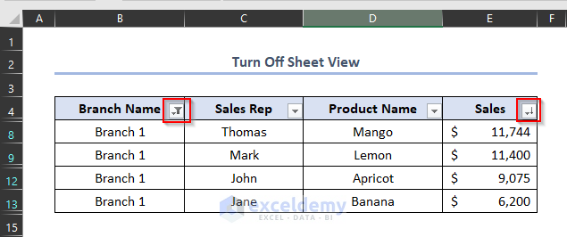
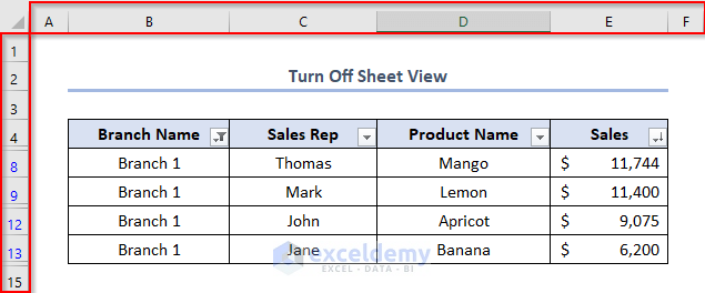
Step 2 – Using Sheet the View Option to Turn Off Sheet View
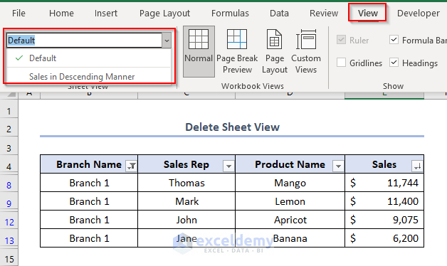
In the following dataset (Turn Off Sheet View), Branch 1 was filtered in the Branch Name header. Sales were filtered in descending order.
To turn off the sheet view:
- Go to View > click Exit in Sheet View.
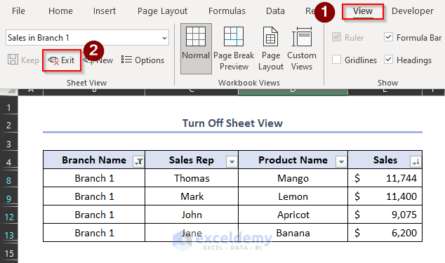
- The sheet view changes to Default view.
Black was removed from Columns and Rows.
Read More: How to Use Sheet View in Excel
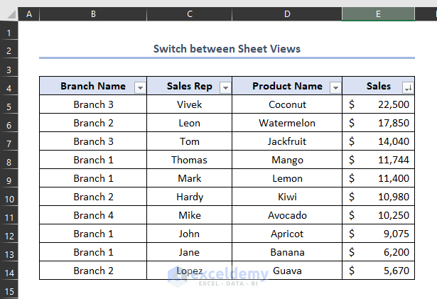
How to Switch Between Sheet Views
Consider the following dataset:
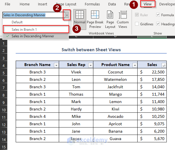
- Go to View. In Sheet View, you’ll see Sales in Descending order.
- Click the icon of the sheet view name.
- Choose any option. Here, Sales in Branch 1 to switch from Sales in Descending Order to Sales in Branch 1.
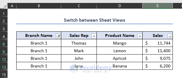
The sheet view is switched to Sales in Branch 1.
How to Delete the Sheet View
Consider the following dataset.
To delete the sheet view Sales in Branch 1:

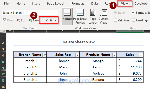
- Go to View > select Options.
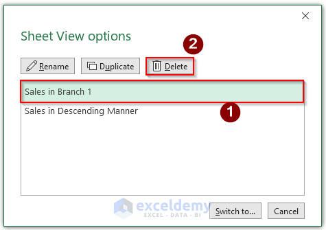
- In Sheet View Options window, choose Sales in Branch 1.
- Click Delete.
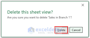
- In the Delete this sheet view?, click Delete.
- Close the Sheet View Options window.
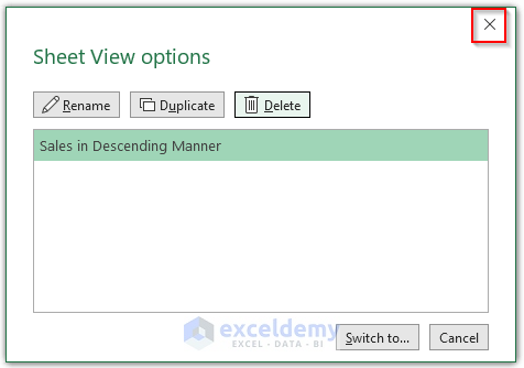
The sheet view of Sales in Branch 1 was deleted. If you go to View, you’ll not see a Sales in Branch 1 option in the Sheet View box.
Download Practice Workbook
<< Go Back to View in Excel | Learn Excel
Get FREE Advanced Excel Exercises with Solutions!

Thank you for your helpful information! – but I have been unable to delete something that I inadvertently created that is related to Sheet View, and I cannot (yet) find help on-line – yours is the closest!
In trying to filter values in a column, I some how I ended up creating a screen in which two columns are not visible, and the filter button on the column I was working on now has an up-arrow in it. Simultaneously, a new bar appeared across my screen below the “formula bar”, with a box labelled “1” in it. (In trying to work out how to removed it, I may have created a second box with a “2” in it – which is there now; but it is possible that it appeared at the same time as Button 1.)
These two boxes are buttons, and I can use them to toggle back-and-forth between the two ways of viewing my data, i.e., in its original state: Button 1 hides 2 columns, and Button 2 returns to normal viewing, with all columns visible. (I can appreciate the potential utility of this feature, but not for my current work.)
Also, a line appears in the new bar, over the two columns that can be hidden, and has a box with a “-” or “+” sign to the right: clicking on one of these (as with clicking on the “1” or “2” buttons to the far left) hides/reveals the hidden columns.
I cannot work out how to delete these buttons and the “hidden columns” feature that I accidentally set up when trying to filter data in a column. I have experimented with “features in the top-level “View” option, and “Screen View” (when in View), and also looked at the filter feature – but no joy.
Is this something that you know how to delete?
Appreciate any advice that you might have!
Sincerely,
Brian
Hello BRIAN
Your appreciation means a lot us. Thanks for reaching out and posting a well-layout question. You encounter an issue with hidden columns and buttons that toggle between different sheet views. And you want to delete these buttons and the hidden column features. It isn’t easy to give an exact solution without the exact details of the worksheet views. However, I have some general ideas to help you with your problem.
First, identify the toggle buttons and go to sheet views, followed by view options. Later, delete that sheet view. Additionally, you remove the applied filters and groupings. Select the columns surrounding the hidden ones, right-click, and choose Unhide to ensure all columns are visible.
If you still have difficulties, you can share your problem in the ExcelDemy Forum with more detailed information. Good luck!
Regards
Lutfor Rahman Shimanto
ExcelDemy