How to Use Sheet View in Excel (with Simple Steps)

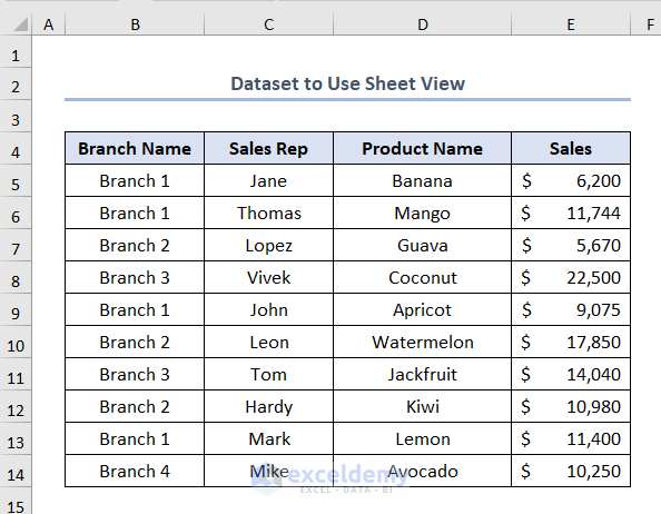
We have made a dataset to use the Sheet View ribbon. It has column headers: Branch Name, Sales Rep, Product Name, and Sales.

Step 1 – Activate Sheet View in Excel

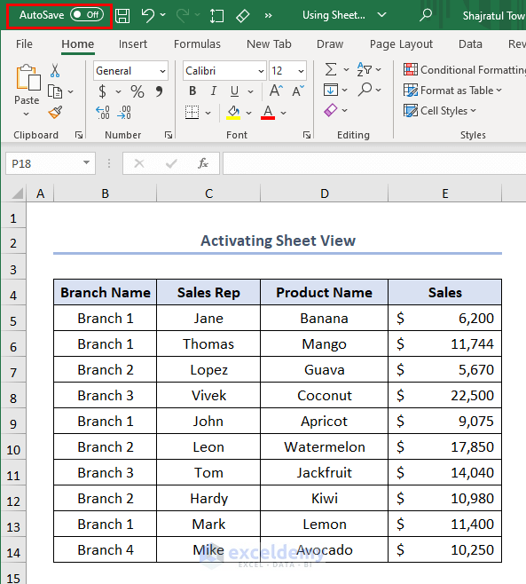
We have to activate Sheet View by saving the Excel sheet in Sharepoint or One Drive. This only works in Excel 365.

• Turn on AutoSave by clicking its button from Off to On.

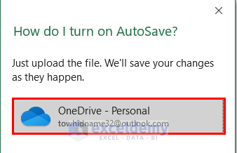
A bar named How do I Turn on AutoSave will appear.

• Select OneDrive – Personal.
• Enter account credentials if needed.

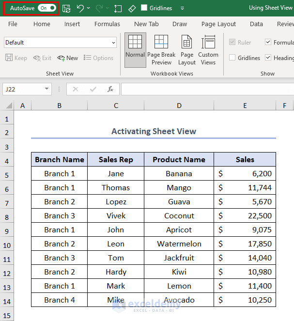
The AutoSave option is turned on now.

Step 2 – Creating a Temporary View for the Sheet View in Excel

• Go to View and click the eye icon in Sheet View.

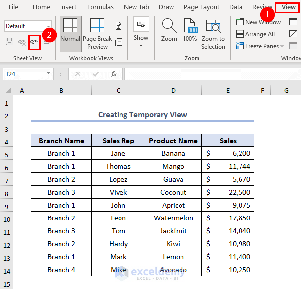
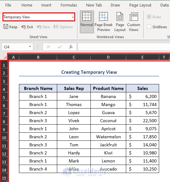
A Temporary View is added.

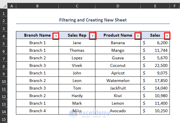
Step 3 – Filtering and Creating a New Sheet

• To bring up the Filter option, click Ctrl + Shift + L. Drop-down arrows will be added like in the picture shown below.

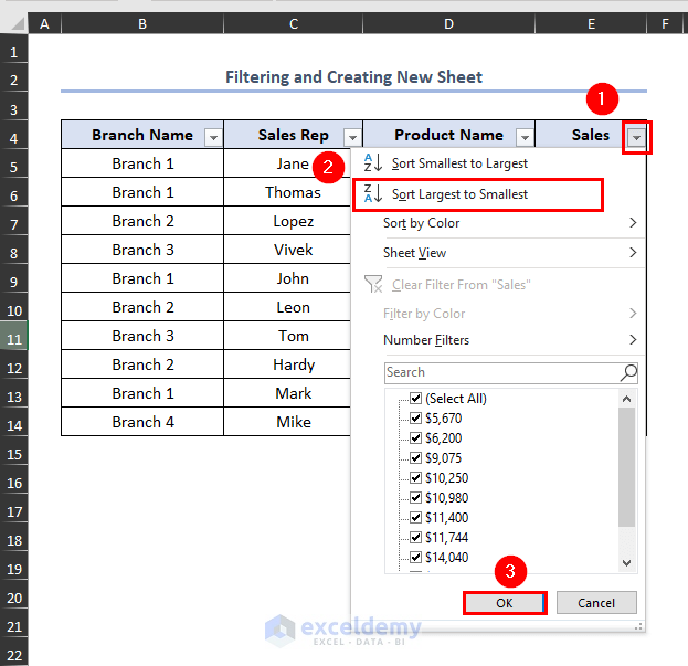
Suppose we want to reorder Sales in descending value.

• Select the Filter option icon in the Sales
• Choose Sort Largest to Smallest.
• Click OK.

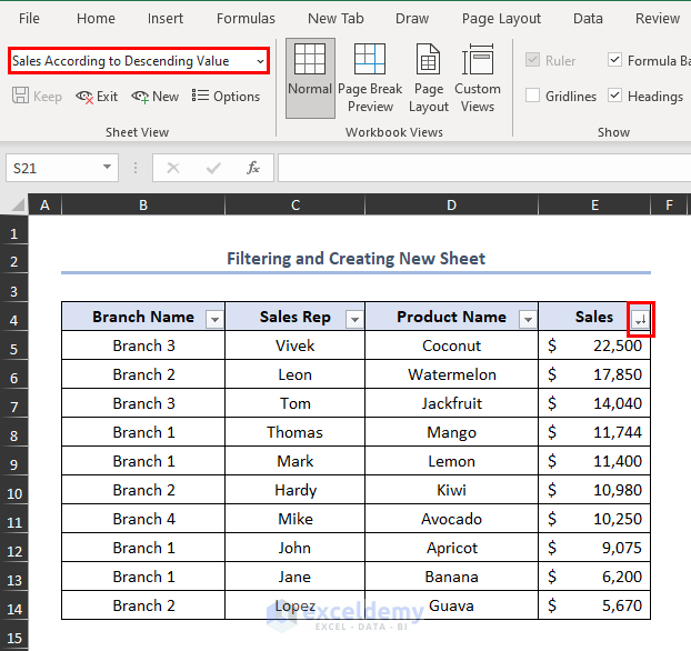
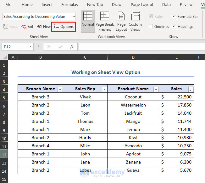
We’ll see that the Sales values are reordered in descending order and the icon of the Sales column is changed which actually indicates that this column is sorted.

• Change the title name to Sales According to Descending Value.

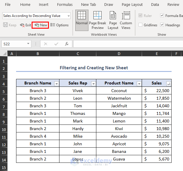
We want to make a sheet of Sales in Branch 1 only.

• Click New from the Sheet View

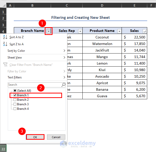
• Select the filter option icon in the Branch Name
• Select Branch 1.
• Click OK.

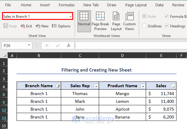
A new sheet will appear.

• Change the title name to Sales in Branch 1.

Step 4 – Working with the Sheet View Option in Excel

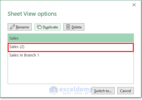
We can Rename, Make Duplicate, or Delete any sheet by using Options from the Sheet View box.

• Click Options.

A Sheet View Options window will appear.

• To Rename the sheet of Sales According to Descending Value, click the sheet first and then click Rename.

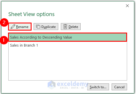
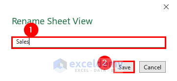
A Rename Sheet View will appear.

• Change the name to Sales.

We want to Duplicate the sheet of Sales.

• Pick the sheet of Sales.
• Select Duplicate.

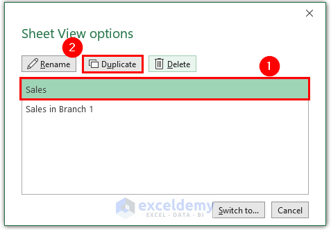
We created Sales (2) as a duplicate sheet of Sales.

• We can delete any sheet in the sheet view by selecting Delete in the Sheet View Option.

Download the Practice Workbook

Related Article

• How to Turn Off Sheet View in Excel

<< Go Back to View in Excel | Learn Excel