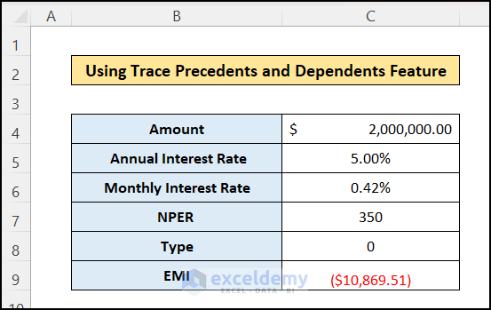
What Are Trace Precedents and Trace Dependents Features in Excel?
In Excel, we use formulas with cell references, and thus, the formula cell becomes dependent on those cells. Trace precedent and dependent features help you to show the relation between the cells.
Trace Precedent:
This feature will show the cells affecting the active cell value. There will be an arrow from the controlling cells to the result cells to identify the trace precedents. Suppose you have selected a cell C13 with the formula “=SUM(C8:C12)”. Then, the cell range C8:C12 is the trace precedent for the active cell.
Trace Dependent:
This feature will show the dependent cells of a cell or the cells where cell references are created using the selected cell. In other words, trace dependent feature identifies the cells affected by the selected cell. Suppose you have selected a cell C13 with the formula “=SUM(C8:C12)”. Now, if you select cell C8 and want to identify the trace dependents of this cell, then it will show up in cell C13.
We must prepare the dataset with the appropriate formula and cell references according to your needs. You may need to use trace precedents or dependents to showcase the relationship between the cells.
Using Excel Trace Precedents Feature
Steps:
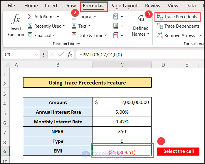
- Select the cell you want to show trace precedents. It will be the active cell.
- Go to the Formulas tab on the top ribbon.
- In the Formula Editing menu, select the Trace Precedents.
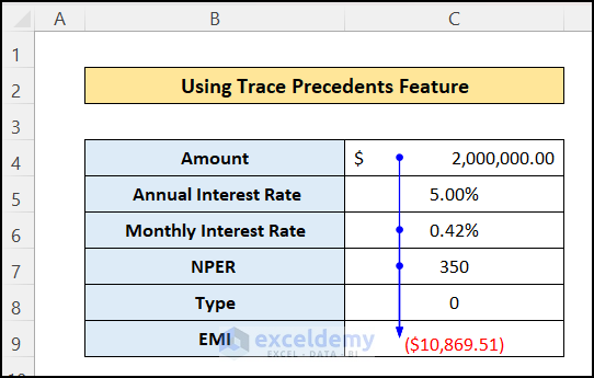
- As a result, you will see that there will be a blue arrow that is directed to the active cell with some bold dots in it.
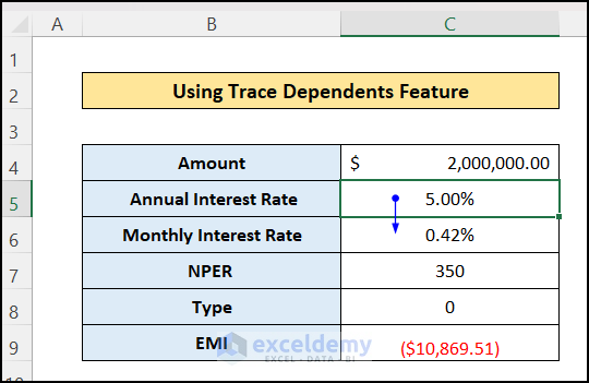
Using the Trace Dependents Feature in Excel
Steps:
- Select the cell you want to identify the trace dependents.
- Go to the Formulas tab in the top ribbon.
- Select the Trace Precedents option in the Formula Editing menu.
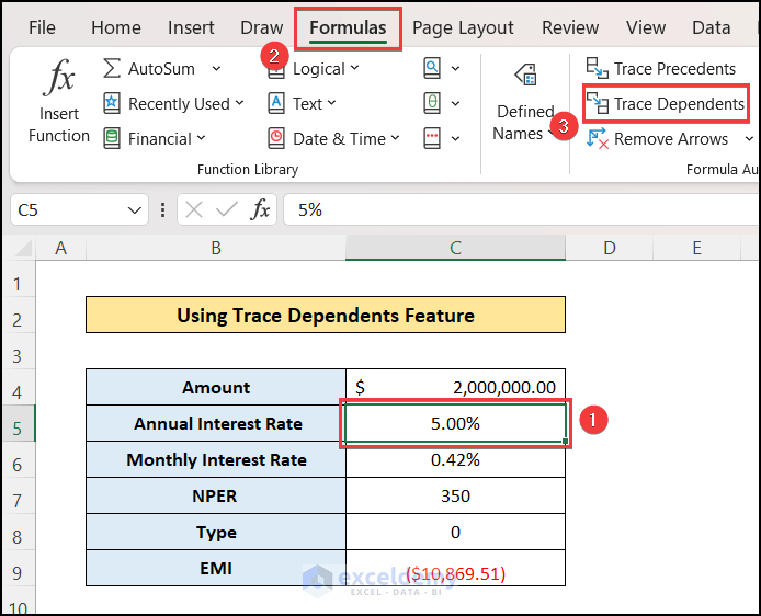
- There will be blue arrows from the active to the dependent cells. You can trace the dependent cells of the active cells in the active Excel worksheet.
Shortcuts for Trace Precedents and Dependents Feature
Steps:
- Select the cell.
- Click the shortcut keys as shown below:
Trace Precedents Shortcut
Alt+T+U+T
Trace Dependents Shortcut
Alt+T+U+D
Read More: How to Trace Dependents Across Sheets in Excel
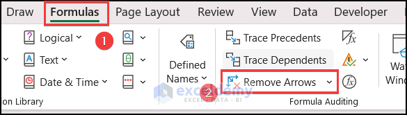
Remove a Trace Arrow or Blue Arrow from the Excel Worksheet
Steps:
- Go to the Formula tab in the top ribbon.
- Select the “Remove Arrows” option, and you will see that all arrows will be removed.
Download the Practice Workbook
You can download the practice workbook from here:
Related Articles
<< Go Back to Trace Formula | Auditing Formulas | Excel Formulas | Learn Excel
Get FREE Advanced Excel Exercises with Solutions!
