How to Trace Errors in Excel – Quick Steps

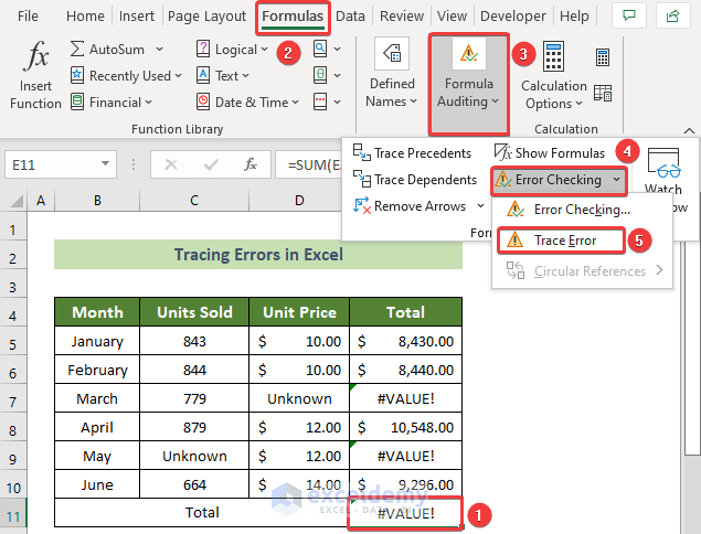
To trace errors in Excel:

Click the error cell >> go to Formulas >> Formula Auditing >>  Error Checking >> Trace Error.

Types of Errors in Excel

#VALUE! :  occurs when you pass an incorrect argument or reference inside a formula. It also occurs when you use the wrong operator or use text instead of numbers inside a formula.

#DIV/0 :  happens if you divide a cell or number by 0 or a blank cell.

#NUM! : occurs if the number inside a cell is too large or too narrow.

#REF! : occurs due to incorrect or missing references.

#N/A : conveys the message Not Available.

 #NAME? : occurs due to wrong spelling or using unavailable table or range names.

#NULL! : occurs if you use an intersection operator between ranges that do not intersect.

How to Trace Errors in Excel

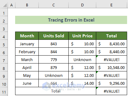
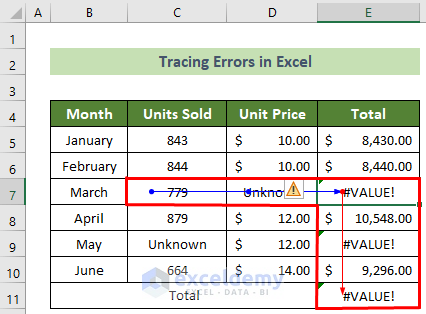
The dataset below contains units sold and unit price of a product over 6 months.

Read More: Excel VBA Watch Window

Steps:

• Click the error cell (E11, here).

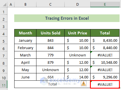
• A yellow marked triangle is displayed on the left side of the cell.
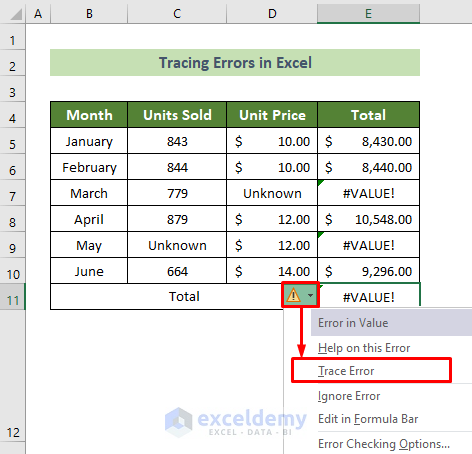
• Hover over the symbol.
• Click the down arrow in the symbol.
• Choose Trace Error.

You will see the error tracing arrows.

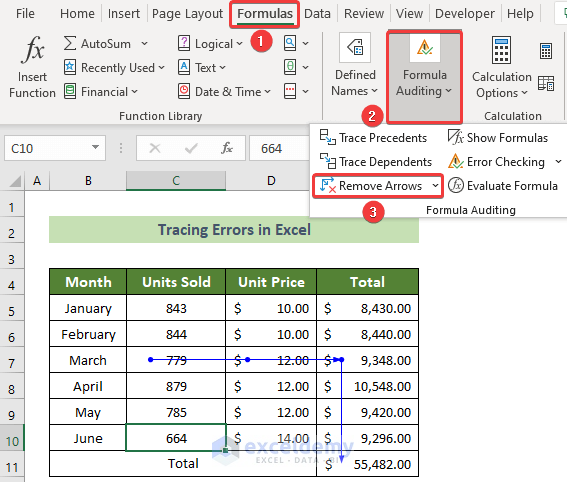
You  can also use the Formulas tab:

• Click E11 >> Go to the Formulas tab >> Formula Auditing >> Error Checking >> Trace Error.

You will see cells causing errors connected by arrows.

How to Remove Error Tracing Arrows in Excel

 Steps:

• Go to the Formulas tab.
• Select Formula Auditing.
• Click Remove Arrows.

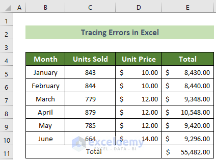
This is the output.

Read More: How to Monitor Cells Using Excel Watch Window

Things to Remember

Error cells have green triangles at the top left corner.

Download Practice Workbook

Download the practice workbook.

<< Go Back to Trace Formula | Auditing Formulas | Excel Formulas | Learn Excel