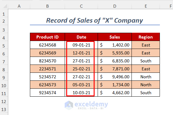
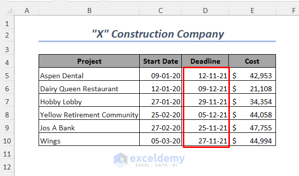
We have two datasets: a company’s Record of Sales, and the records for construction company X, containing different projects and their costs.
Method 1 – Using the SUMIFS function for a Date Range of a Month
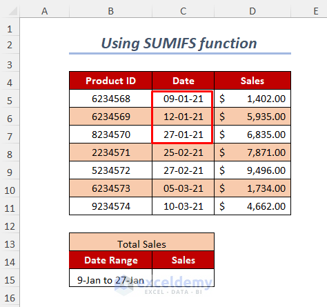
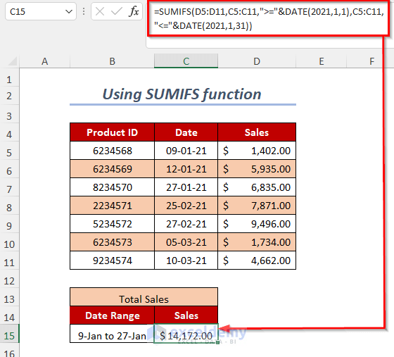
If you want to add the sales for a date range of January month then you can use the SUMIFS function and the DATE function.
Steps:
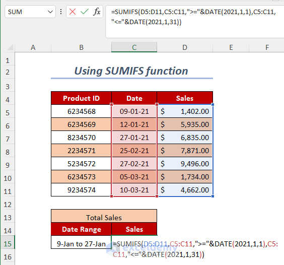
- Enter the following formula in cell C15:
=SUMIFS(D5:D11,C5:C11,">="&DATE(2021,1,1),C5:C11,"<="&DATE(2021,1,31))D5:D11 is the range of Sales, and C5:C11 is the criteria range which includes the Dates.
">="&DATE(2021,1,1) is the first criterion where DATE will return the first date of a month.
"<="&DATE(2021,1,31) is used as the second criterion where DATE will return the last date of a month.
- Press ENTER.
Now, you will get the sum of sales for a date range of 9 January to 27 January.
Method 2 – Combining the SUMIFS function and EOMONTH function
Steps:
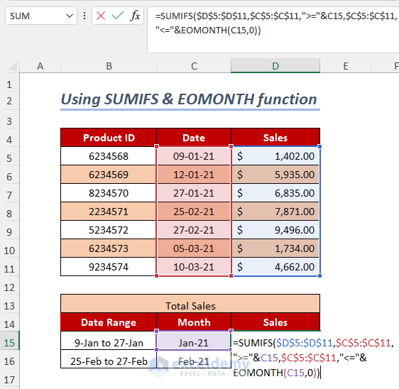
- Enter the following formula in cell D15:
=SUMIFS($D$5:$D$11,$C$5:$C$11,">="&C15,$C$5:$C$11,"<="&EOMONTH(C15,0))$D$5:$D$11 is the range of Sales, $C$5:$C$11 is the criteria range
">="&C15 is the first criteria, where C15 is the first date of a month.
"<="&EOMONTH(C15,0) is used as the second criterion, where EOMONTH will return the last date of a month.
- Press ENTER.
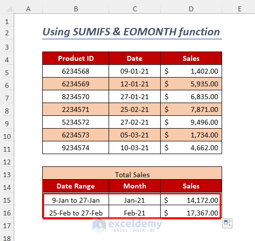
- Drag down the Fill Handle tool.
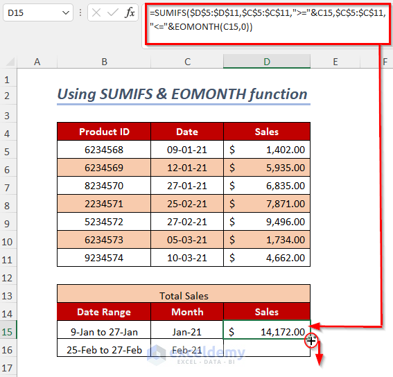
You will get the sum of sales for different date ranges of January and February.
Read More: Sum Values Based on Date in Excel
Method 3 – Applying the SUMPRODUCT function
Steps:
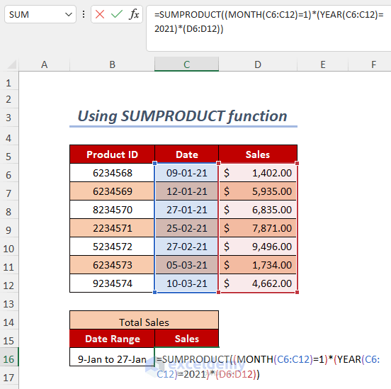
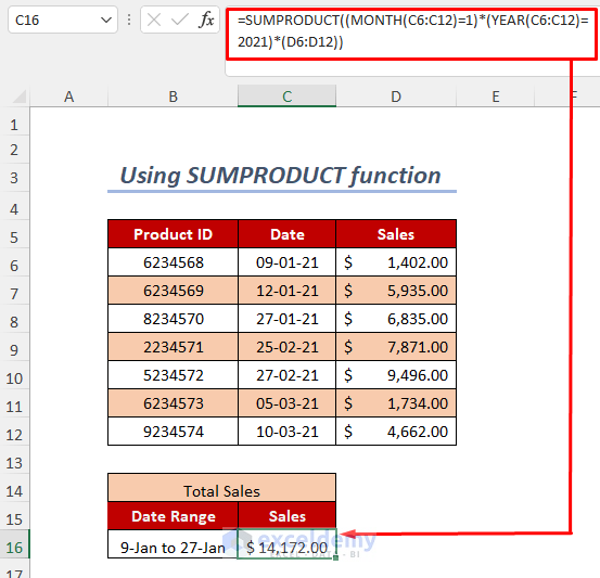
- Type the following formula in cell C16:
=SUMPRODUCT((MONTH(C6:C12)=1)*(YEAR(C6:C12)=2021)*(D6:D12))D6:D12 is the range of Sales, and C6:C12 is the range of Dates.
MONTH(C6:C12)will return the months of the dates, and then it will be equal to 1 and it means January.
YEAR(C6:C12)will provide the years and dates, and it will be equal to 2021.
- Press ENTER.
You will get the sum of sales for a date range of 9 January to 27 January.
Method 4 – Summing up Values for a Date Range of a Month based on Criteria
Steps:
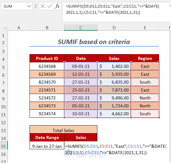
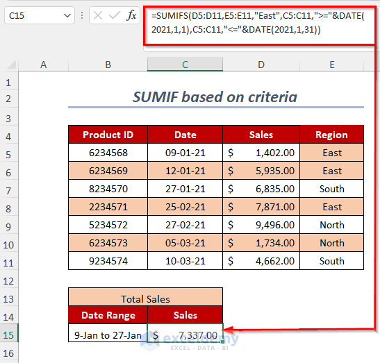
- Enter the following formula in cell C15:
=SUMIFS(D5:D11,E5:E11,"East",C5:C11,">="&DATE(2021,1,1),C5:C11,"<="&DATE(2021,1,31))D5:D11 is the range of Sales, E5:E11 is the first criteria range and C5:C11 is the second and third criteria range.
East is used as the first criterion.
">="&DATE(2021,1,1) is the second criterion where DATE will return the first date of a month.
"<="&DATE(2021,1,31) is used as the third criterion where DATE will return the last date of a month.
- Press ENTER.
You will get the sum of sales for a date range of 9 January to 27 January for the East Region.
Method 5 – Combining SUM and IF Functions for Date Range of a Month Based on Criteria
Steps:
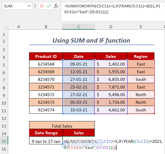
- Enter the following formula in cell C15.
=SUM(IF(MONTH(C5:C11)=1,IF(YEAR(C5:C11)=2021,IF(E5:E11="East",D5:D11))))For the IF function, three logical conditions have been used here that will match the desired date range and the criteria for the East Region.
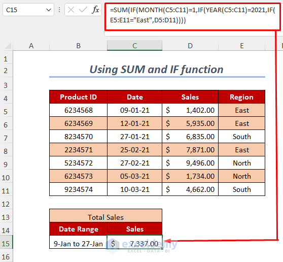
- Press ENTER.
You will get the sum of sales for a date range of 9 January to 27 January for the East Region.
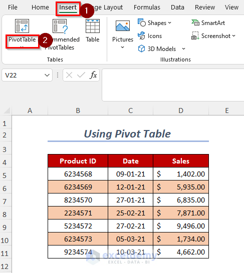
Method 6 – Utilizing Excel Pivot Table
Steps:
- Go to Insert Tab>>PivotTable option.
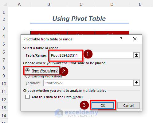
Create PivotTable Dialog Box will pop up.
- Select the table/range.
- Click on New Worksheet.
- Press OK.
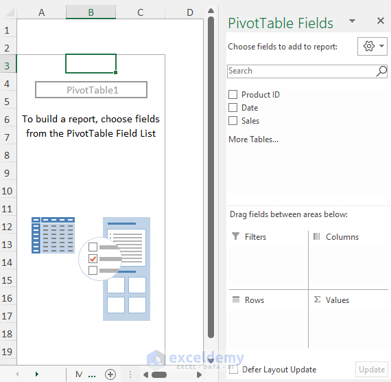
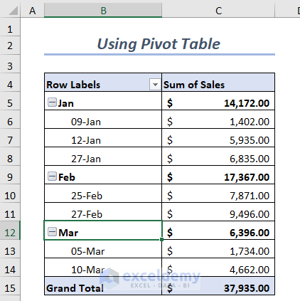
Then a new sheet will appear where you have two portions named PivotTable1 and PivotTable Fields.
- Drag down the Date to the Rows area and Sales to the Values area.
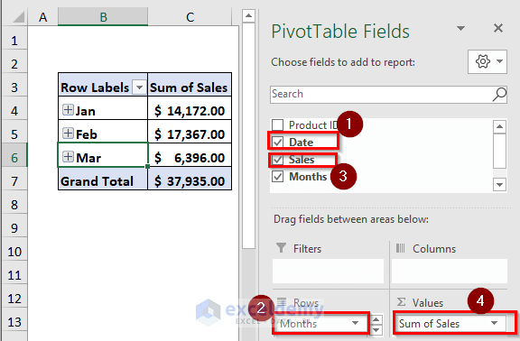
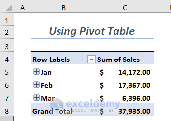
The following table will be created.
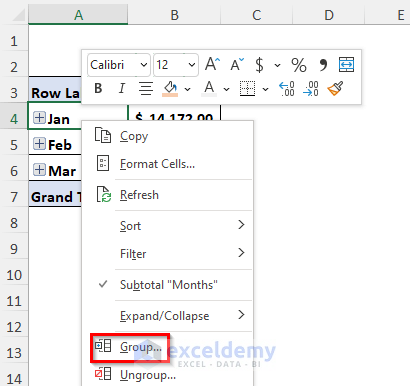
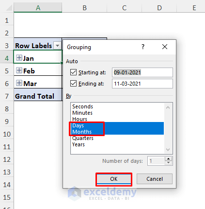
- Select any cell of the Row Labels column.
- Right-click.
- Choose Group Option.
- Click on the Days and Months option in the indicated area.
- Press OK.
You will get the sum of sales for a range of dates of a month as below.
Method 7 – Using the SUMIF Function Based on Empty or Non-Empty Dates
Case 1: Total Cost for Non-Empty Dates
Steps:
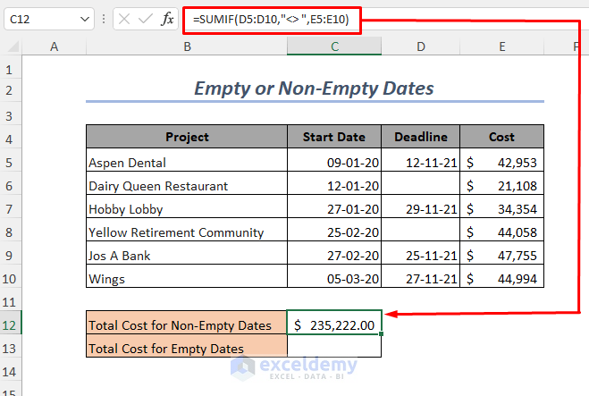
- Enter the following formula in cell C12:
=SUMIF(D5:D10,"<> ",E5:E10)E5:E10 will give the range of Sales.
D5:D10 is the range of Dates.
“<> ” means not equal to Blank.
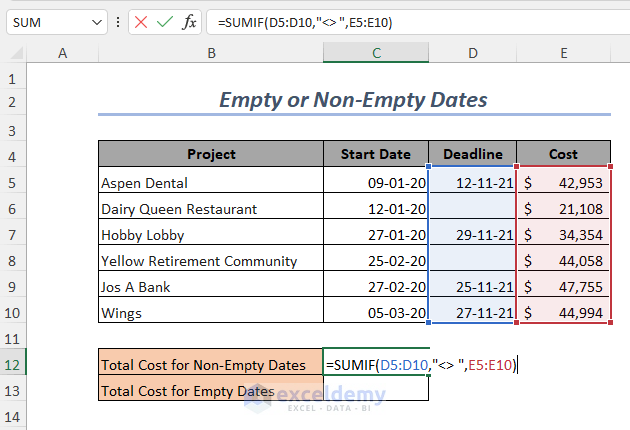
- Press ENTER.
You will get the Total Cost for Non-Empty Dates.
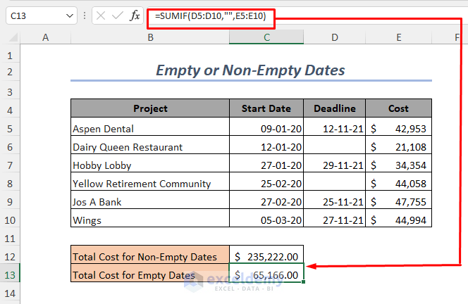
Case 2: Total Cost for Empty Dates
Steps:
- Enter the following formula in cell C13:
=SUMIF(D5:D10,"",E5:E10)E5:E10 will give the range of Sales.
D5:D10 is the range of Dates.
“” means equal to Blank.
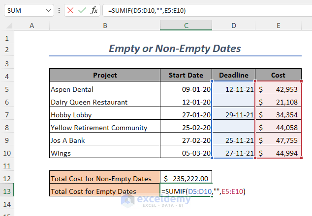
- Press ENTER.
You will get the Total Cost for Empty Dates.
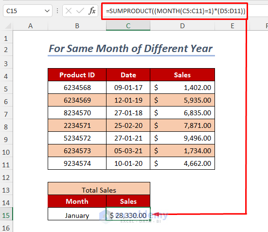
Method 8: Using the SUMPRODUCT Function for the Same Month of Different Years
Steps:
- Enter the following formula in cell C15:
=SUMPRODUCT((MONTH(C5:C11)=1)*(D5:D11))D5:D11 will give the range of Sales.
MONTH(C5:C11)=1 is for January month.
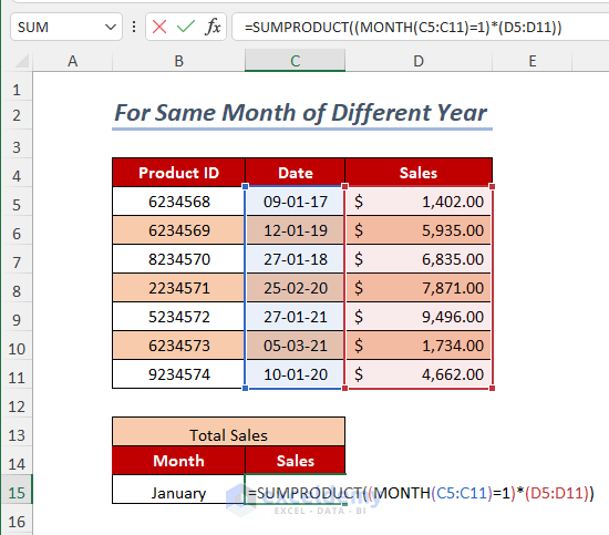
- Press ENTER.
You will get the sum of Sales for January of different years.
Read More: How to Do SUMIF by Month and Year in Excel
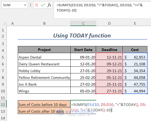
Method 9 – Using the TODAY Function to Sum Up Values
Case 1: Sum of Costs Before 10 Days from Today
Steps:
- Enter the following formula in cell C12:
=SUMIFS(E5:E10, D5:D10, "<"&TODAY(), D5:D10, ">="&TODAY()-10)TODAY() will give today’s date.
"<"&TODAY() is the first criteria and the second criteria is “>=”&TODAY()-10.
E5:E10 will give the range of Sales.
D5:D10 is the range of Dates.
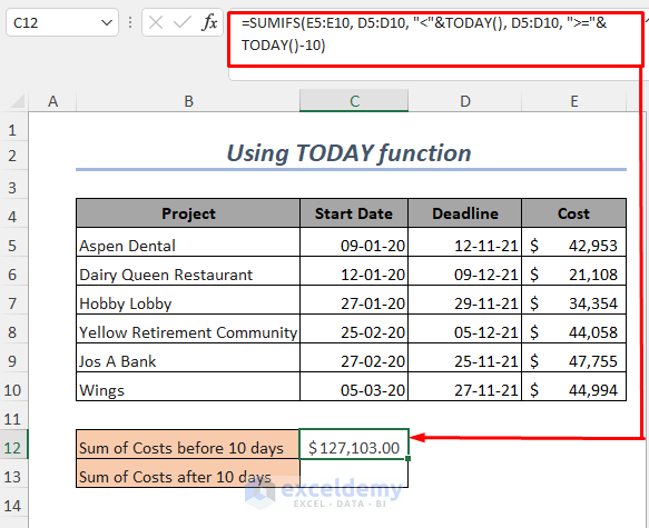
- Press ENTER.
You will get the Sum of Costs before 10 days.
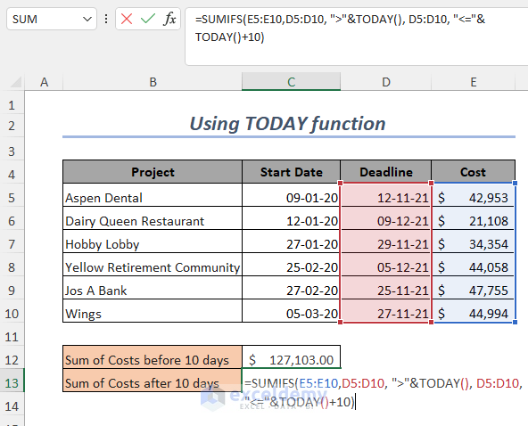
Case 2: Sum of Costs After 10 Days from Today
Steps:
- Enter the following formula in cell C13:
=SUMIFS(E5:E10,D5:D10, ">"&TODAY(), D5:D10, "<="&TODAY()+10)TODAY() will give today’s date.
">"&TODAY() is the first criterion and the second criterion is “<=”&TODAY()+10.
E5:E10 will give the range of Sales.
D5:D10 is the range of Dates.
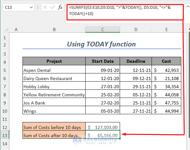
- Press ENTER.
You will get the Sum of Costs after 10 days.
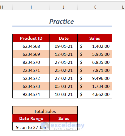
Practice Section
We have provided a Practice section for each method.
Download the Practice Workbook
<< Go Back to SUMIF Date Range | Excel SUMIF Function | Excel Functions | Learn Excel
Get FREE Advanced Excel Exercises with Solutions!
