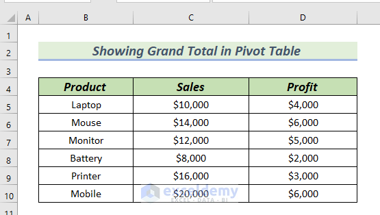
The following dataset has the Product, Sales, and Profit columns. Using this sample dataset, we will insert a Pivot Table.
Method 1 – Using Grand Totals Feature in Pivot Table
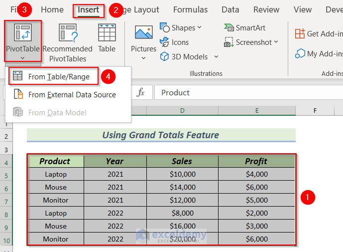
We will use the Grand Total feature to show Grand Total in Pivot Table. A Year column is added in the dataset. The Year column contains 2 types of years. The Product column has 3 types of products.
Step 1: Inserting Pivot Table
- Select the entire dataset.
You can select the entire dataset by clicking on cell B4 and pressing the CTRL+SHIFT+Down arrow.
- Go to the Insert tab.
- From the PivotTable group >> select From Table/Range.

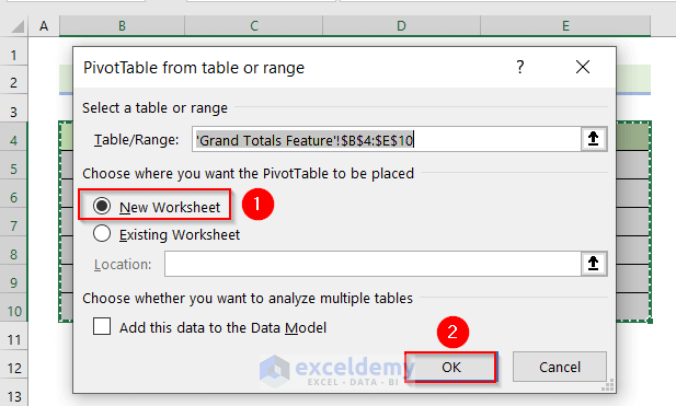
A PivotTable from table or range dialog box will pop up.
- Select New Worksheet >> click OK.
As a result, you will see PivotTable Fields in a different worksheet.
- We will mark the Product >> drag it to the Rows group.
- We will mark the Sales >> drag it to the Values group.
- We mark the Year >> drag it to the Column group.

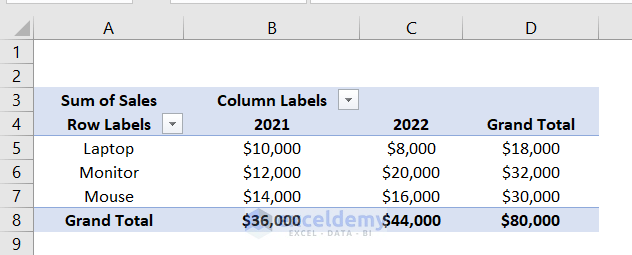
You will see that the Pivot Table has been created.
Step 2: Use of Grand Totals Feature
In the above Pivot Table, the Grand Total has been created automatically.
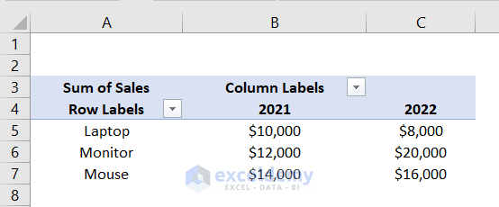
If the Pivot Table looks like the following image where the Grand Total for rows and columns is missing, we have to use the Grand Totals feature.
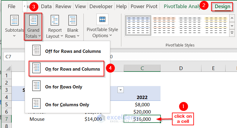
- Click on any of the cells of the Pivot Table.
- From the Design tab >> select Grand Totals.
- Select the on for Rows and Columns option.
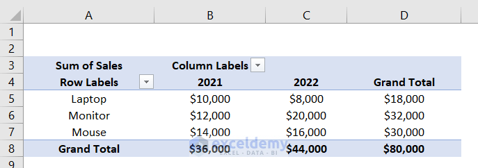
The Pivot Table will show Grand Total for rows and columns.
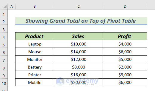
Method 2 – Showing Grand Total on Top of Pivot Table
The following dataset has the Product, Sales, and Profit columns. Using this dataset, we will insert a Pivot Table. After that, we will show grand total on top of the Pivot Table.
Step 1: Inserting Pivot Table
- Create the Pivot Table following Step 1 of Method 1.
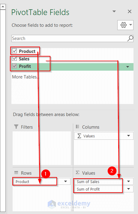
- In the PivotTable Fields, mark the Product >> drag it to the Rows group.
- Select the Sales and Profit >> drag them to the Values group.
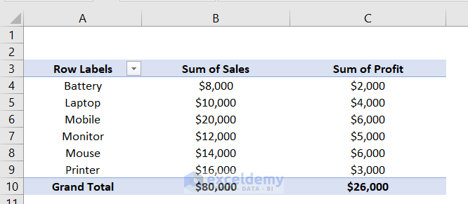
In the Pivot Table, you will notice that the Grand Total is at the bottom of the Pivot Table.
Step 2: Adding Grand Total Column in Source Data
- Select Column C >> right-click on it.
- Select Insert from the Context Menu.
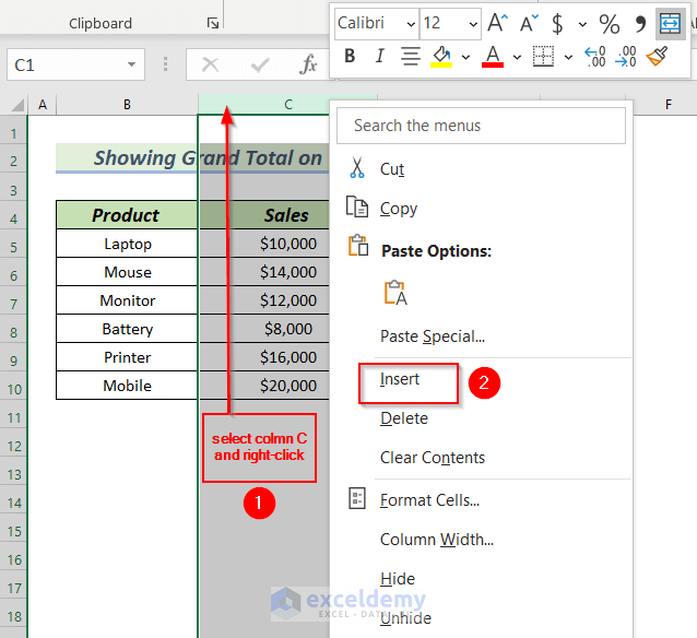
A new column will be inserted into the Dataset.
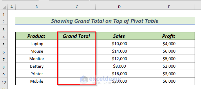
- Name the column, Grand Total.
Leave the column Grand Total empty.
Step 3: Showing Grand Total on Top of Pivot Table
- Go back to the Pivot Table.
- Right-click on any cell of the Pivot Table >> select Refresh from the Context Menu.
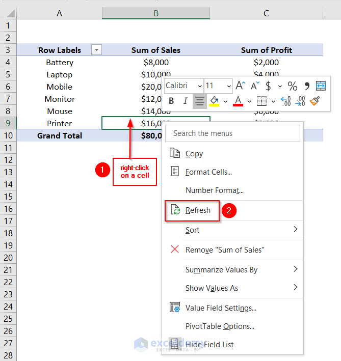
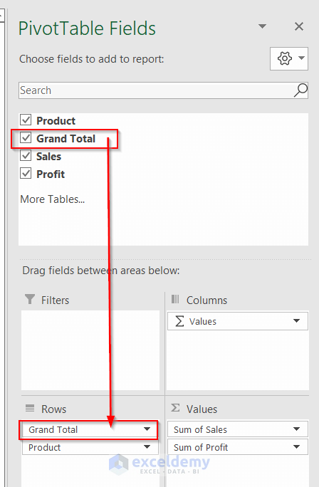
The result will show the Grand Total in the PivotTable Fields.
- Select Grand Total >> drag it in the Rows group above the Product.
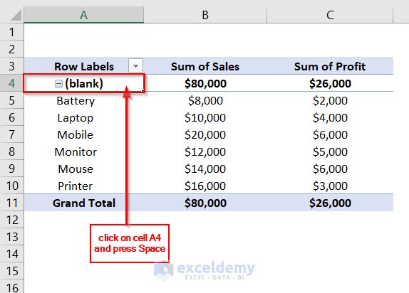
You will see the blank in cell A4.
The grand total of Sales is in cell B4 and grand total of Profit is in cell C4.
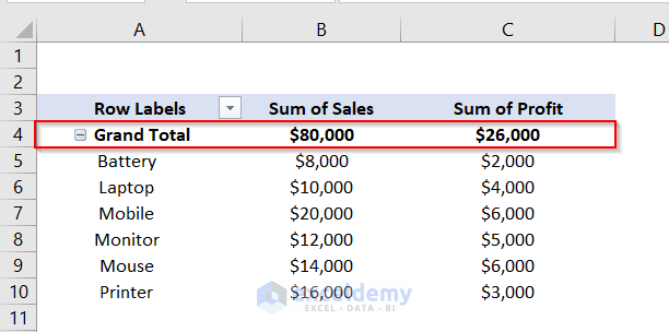
- Click on cell A4 and press the Space bar of the Keyboard.
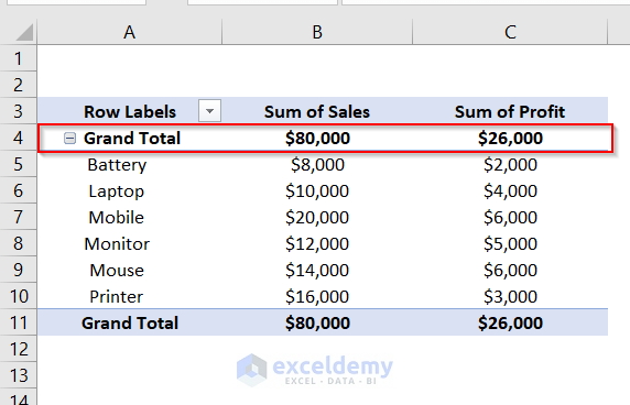
- Enter Grand Total in cell A4.
Grand Total will show at the top of the Pivot Table.
If you do not want Grand Total at the bottom of the Pivot Table.
- Right-click on the Grand Total of cell A11.
- Select Remove Grand Total from the Context Menu.
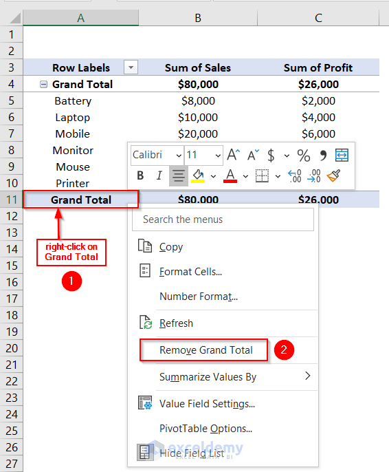
The Grand Total will be at the Top of the Pivot Table.
Read More: How to Remove Grand Total from Pivot Table
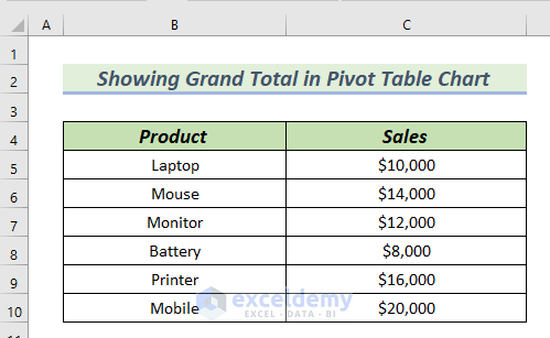
Method 3 – Showing Grand Totals in Pivot Table Chart
Using the following dataset, we will insert a Pivot Table and insert a Column chart using the Pivot Table.
Step 1: Inserting Pivot Table
- Create the Pivot Table following Step 1 of Method 1.
- In the PivotTable Fields, mark the Product >> drag it to the Rows group.
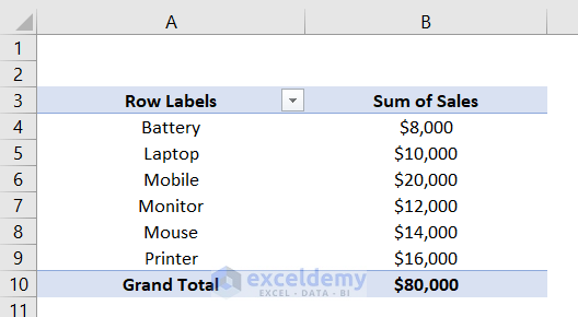
- Select the Profit >> drag it to the Values group.
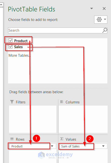
The Pivot Table will be created.
Step 2: Inserting Column Chart
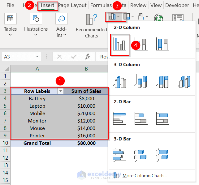
- Select cells A4:B9.
- Go to the Insert tab.
- From the Insert Column or Bar Chart group >> select 2D Clustered Column chart.
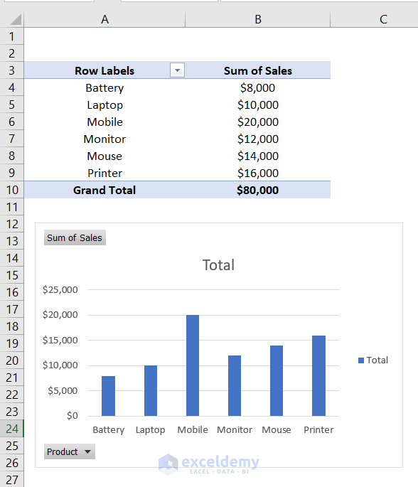
The Column chart will be inserted.
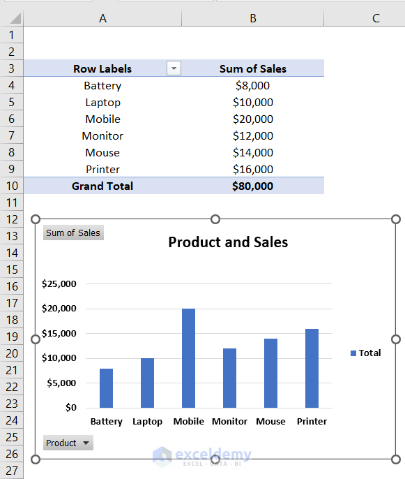
- Rename the Chart Title to Product and Sales.
Step 3: Adding Grand Total to Chart
- In cell D4, enter the following formula.
="Grand Total: "&TEXT(GETPIVOTDATA("Sales",$A$3),"$#,###")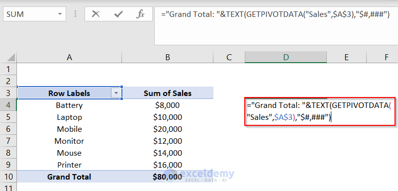
Formula Breakdown
- TEXT(GETPIVOTDATA(“Sales”,$A$3),”$#,###”) → the TEXT function is used to add $ sign before Grand Total.
- Output: $80,000
- “Grand Total: “&TEXT(GETPIVOTDATA(“Sales”,$A$3),”$#,###”) → The ampersand & is used to join “Grand Total: “ with $80,000.
- Output: Grand Total: $80,000
- Press ENTER.
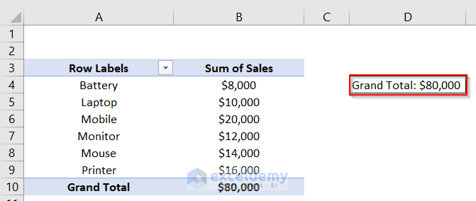
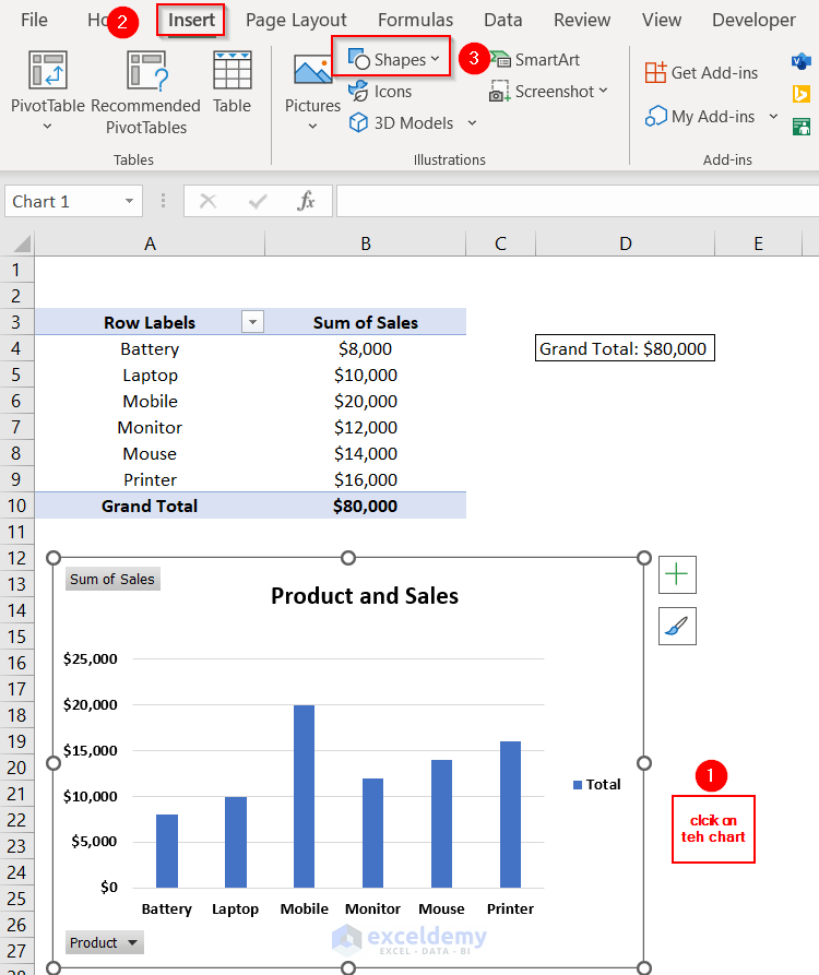
Add the Grand Total to the Chart.
- Click on the Chart >> go to the Insert
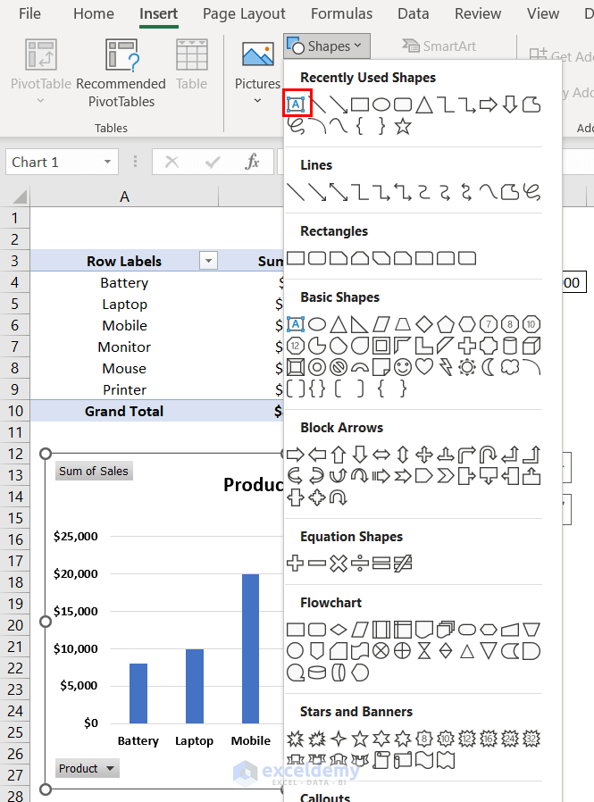
- From the Illustrations group >> select Shapes.
- Select Text Box.
- Insert the Text Box in the chart under the Chart Title.
- In the Formula Bar, enter the following formula.
='Pivot Table Chart'!$D$4 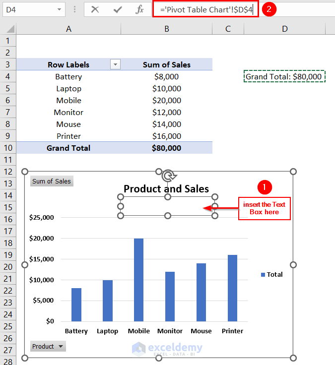
- Press ENTER.
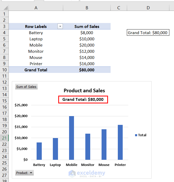
The Grand Total in the chart will be as depicted in the image below.
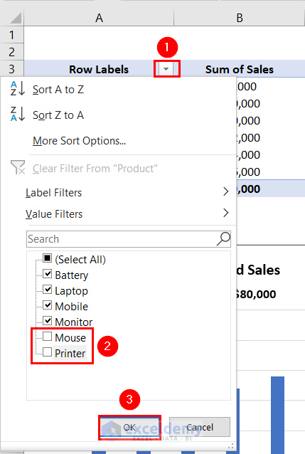
Remove some products from the Grand Total column.
- Click on the drop-down arrow of the Row Labels c
- Unmark the Printer and Mouse.
- Click OK.
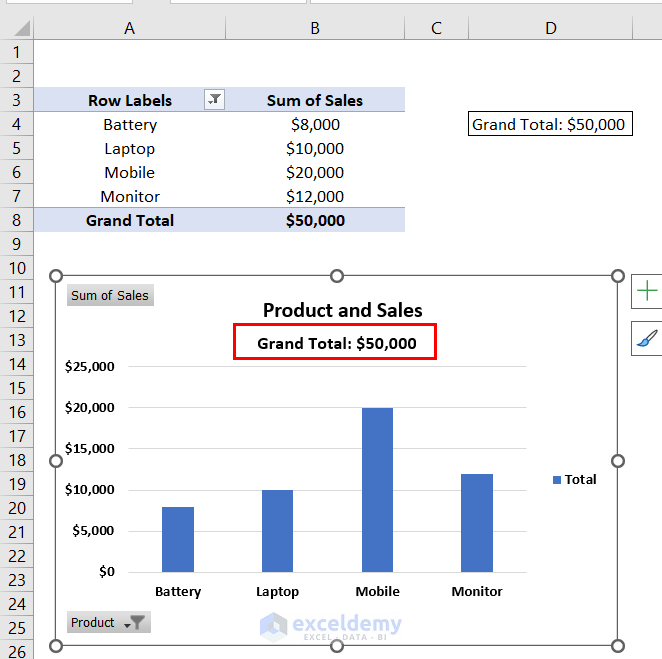
The Grand Total will be changed in the Chart.
Download Practice Workbook
Related Articles
- How to Collapse the Table to Show the Grand Totals Only
- [Fixed!] Pivot Table Grand Total Column Not Showing
<< Go Back to Pivot Table Calculations | Pivot Table in Excel | Learn Excel
Get FREE Advanced Excel Exercises with Solutions!
