To collapse the table and display the Totals only:
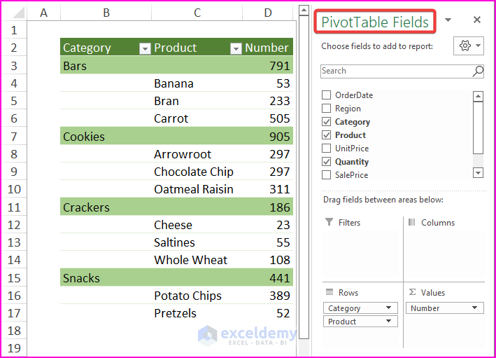
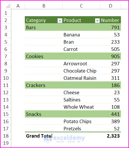
Insert an Excel Pivot Table (Insert > Pivot Tables) to customize data reports, to show or hide details regarding entries and Totals (Subtotals or Grand Totals). To display the Grand Totals:
- Place the Cursor on any cell within the Pivot Table to display the PivotTable Analyze and Design tabs.
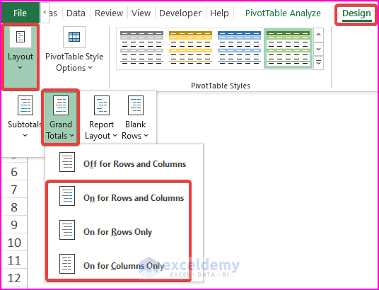
- Click Design and go to the Grand Total section.
- Select one of the 3 options to display the Grand Totals Field inside the Table.
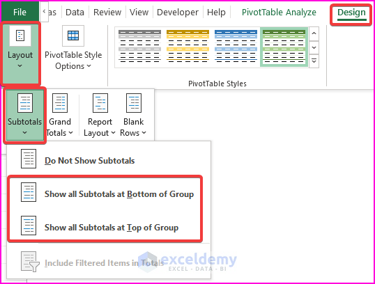
- Repeat the same process to display the Subtotals within the Pivot Table.
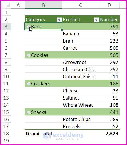
Method 1 – Double-Clicking to Collapse the Table and Show the Grand Totals Only
Steps:
- Double-click any field to hide or collapse product details.
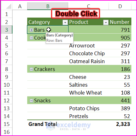
- Repeat the previous step for other fields.
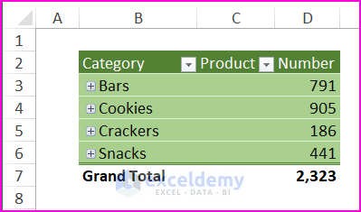
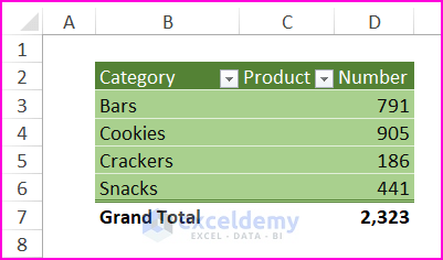
This is the output.

Method 2 – Enabling the Expand/Collapse Button to Collapse Items Within Table
Step 1:
- Select any Pivot Table cells and go to PivotTable Analyze > Show > Click Buttons.
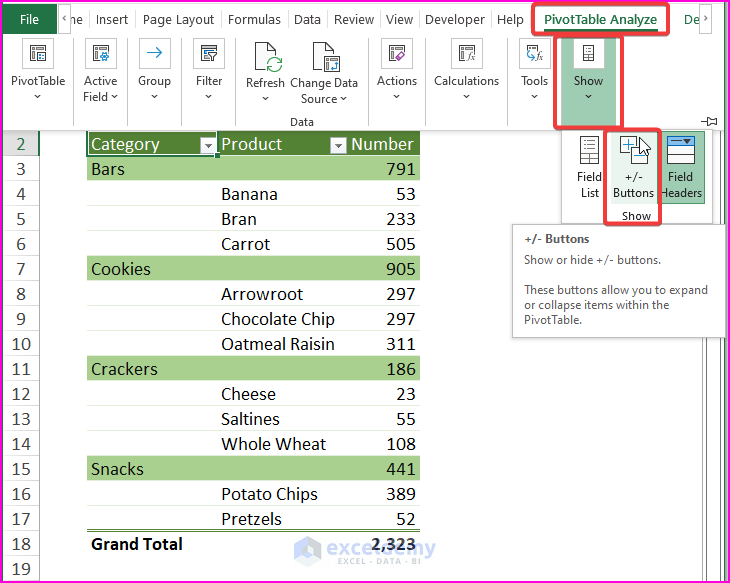
Step 2:
Excel displays the Expand/Collapse Buttons.
- Click them to expand/collapse the table.
This is the output.
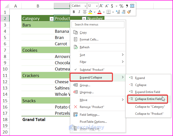
Method 3 – Selecting the Context Menu Option to Show Grand Totals Only
Steps:
- Right-click any field to open the Context Menu.
- Click Expand/Collapse > Collapse Entire Field.
This is the output.
Method 4 – Using Keyboard Shortcuts to Collapse Table Items
Step 1:
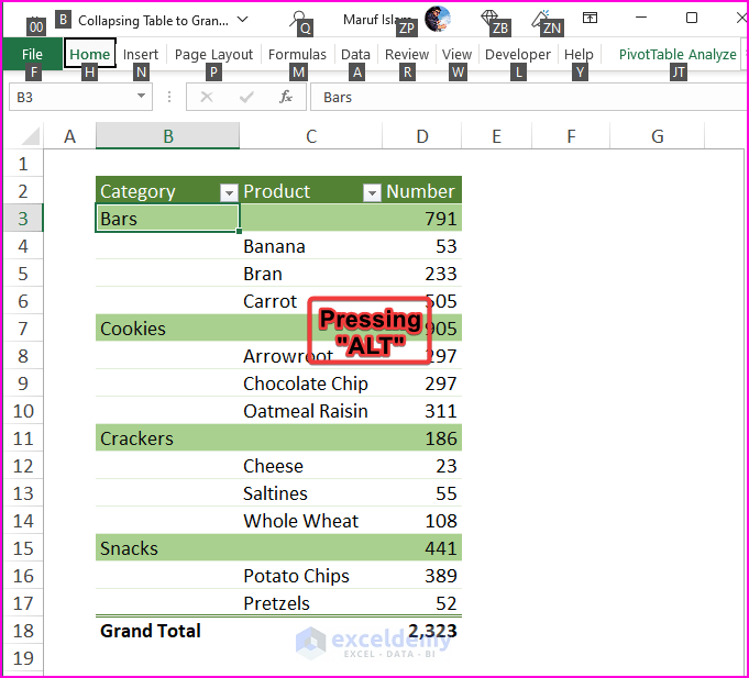
- In the Excel worksheet that contains the Pivot Table, press ALT. Excel displays the key command options.
Step 2:
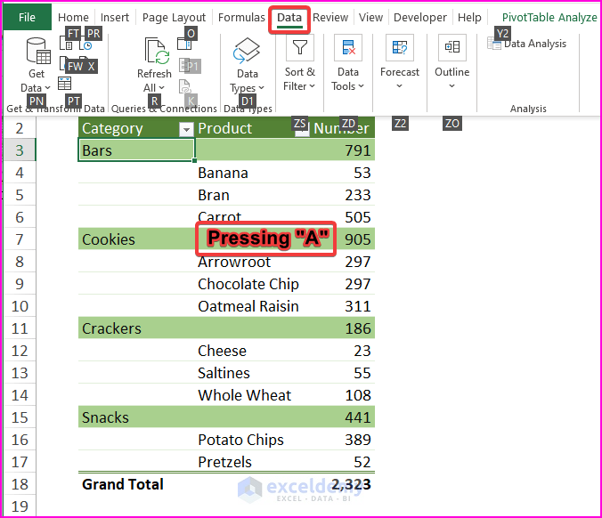
- Press A to select the Data tab.
Step 3:
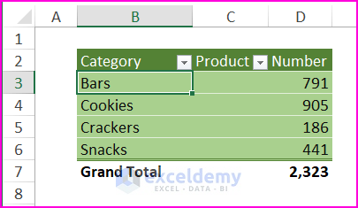
- Press H to collapse the table.
Method 5 – Running a VBA Macro to Display Grand Totals Only
Step 1:
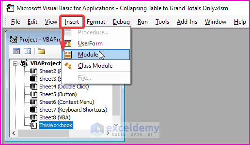
- Press ALT+F11 or go to Developer > Visual Basic to open the Microsoft Visual Basic window.
- Insert a Module by clicking Insert > Module.
Step 2:
- Enter the following macro in the module.
Sub Collapse_Totals_Only()
Dim mPT As PivotTable
Dim mPF As PivotField
Dim mPI As PivotItem
Dim mFieldCount As Long
Dim mPosition As Long
Set mPT = ActiveSheet.PivotTables(1)
mFieldCount = mPT.RowFields.Count - 1
For mPosition = mFieldCount To 1 Step -1
 For Each mPF In mPT.RowFields
  If mPF.Position = mPosition Then
   For Each mPI In mPF.PivotItems
    If mPI.ShowDetail = True Then
     mPF.ShowDetail = False
     Exit Sub
    End If
   Next mPI
  End If
 Next mPF
Next mPosition
End Sub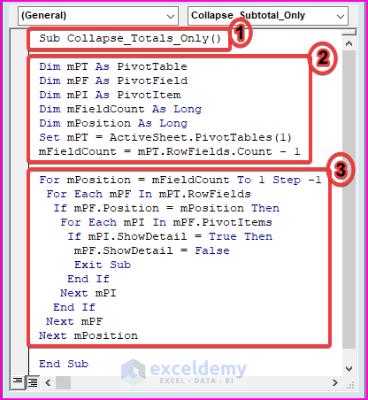
Macro Explanation
activates the macro by setting the Sub name.
declares the variable and assigns the initial value to statements. The row area is deducted by 1, as the last field can’t be expanded.
uses VBA FOR and VBA IF statements to check the Pivot Items’ status and collapses the table to fields.
Step 3:
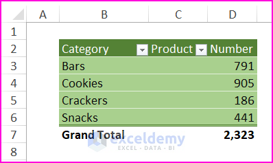
- Run the macro by pressing F5.
- Go back to the worksheet. The entire table collapsed to fields showing the totals only.
Download Excel Workbook
Related Articles
- How to Show Grand Total in Pivot Table
- How to Remove Grand Total from Pivot Table
- [Fixed!] Pivot Table Grand Total Column Not Showing
<< Go Back to Pivot Table Calculations | Pivot Table in Excel | Learn Excel
Get FREE Advanced Excel Exercises with Solutions!
