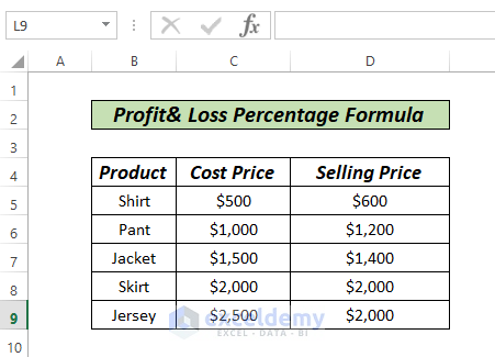
In this article we will cover several simple and effective ways to use a profit and loss percentage formula in Excel. To demonstrate our methods, we’ll use the following sample dataset containing Product, Cost Price, and Selling Price, and calculate the Profit/Loss Amounts and Percentages.
The following general mathematics formula is used to determine the percentage of profit or loss:
= (Gain or loss/previous value*100)
Method 1 – Profit and Loss Percentage Formula from Cost price and Sell Price
In this method, we will use the mathematical formula above to obtain the profit or loss, then use percentage formatting from the Number Format ribbon.
STEPS:
- In cell E5 enter the following formula:
=D5-C5
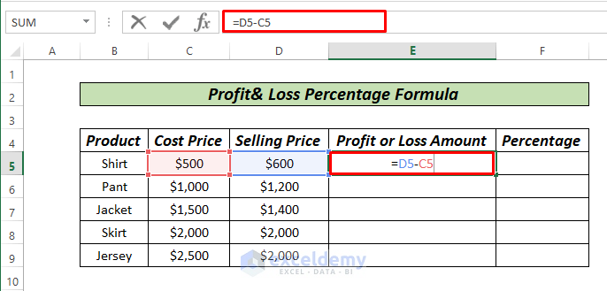
- Press ENTER.
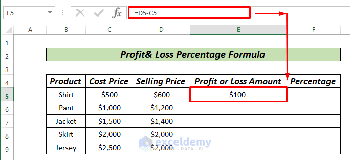 Use AutoFill to fill the rest of the series by right-clicking the mouse button and dragging it down.
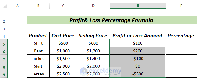
The profit or loss amount is returned, where a positive value indicates Profit and a negative value indicates Loss.
- In cell F5 enter the following formula:
=E5/C5 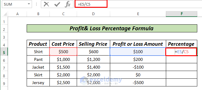 Press ENTER.
- Right-click the mouse button and drag it down to fill the rest of the series.
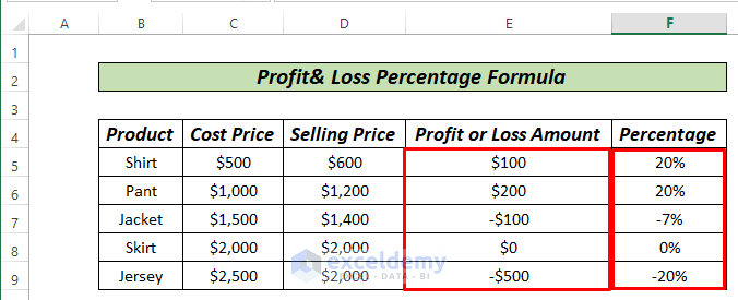
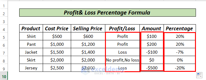
Here, we calculate the amount of profit or loss by subtracting the Cost Price from the Selling Price. Then, we divide the Profit or Loss amount by the Cost Price. Now, we can multiply it by a hundred to get the percentage. Excel has an in-built feature to do this automatically.
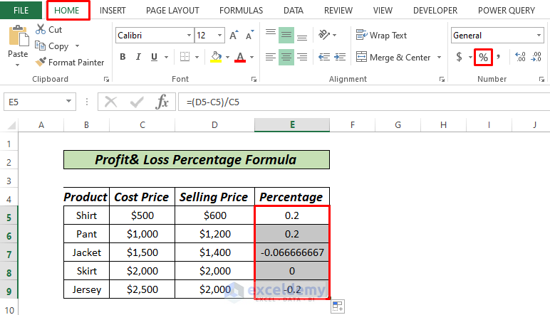
- Select the range from F5 to F9.
- Go to the Home tab and click the Percentage sign (%).
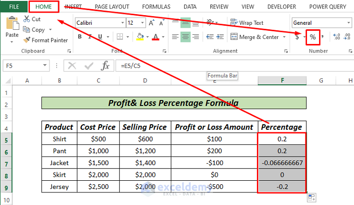
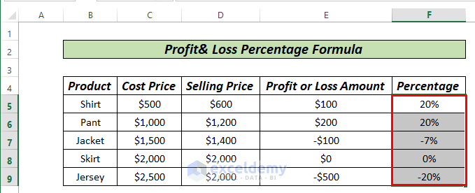
Our result is ready and it looks like the following image.
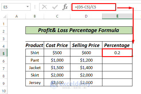
Method 2 – Profit and Loss Percentage Formula in Excel
- In cell F5 enter the following formula:
=(D5-C5)/C5
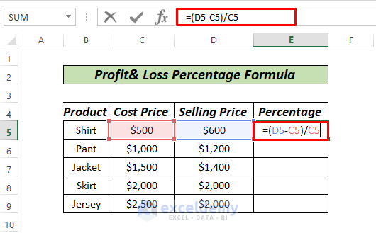
We subtract Cost Price from Selling Price then divide it by the Cost Price to calculate the percentage of profit or loss.
- Press ENTER.
 Drag down to AutoFill.
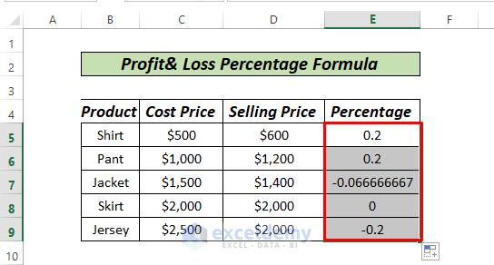 Go to the Home tab and select the Percentage icon.
Our result is returned. A positive value indicates Profit and negative value indicates Loss.
Method 3 – Profit and Loss Percentage Formula with Conditional Formatting
STEPS:
- Follow all the procedures in Method 1.
After completing them, our result will look like this:
 Select the range E5 to E9.
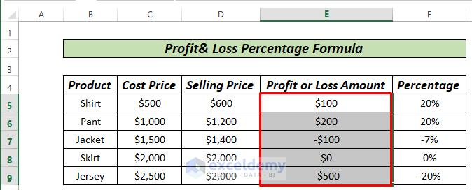 Go to the Home tab, then Conditional Formatting and select New Rule.
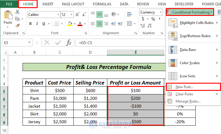 A new dialogue box will pop up.
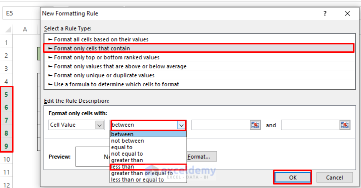
- Select Format only cells that contain.
- In Edit the Rule Description select less than.
- Enter value 0 as we want negative values to be formatted.
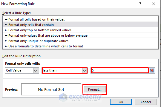 Click on the Format option.
Another dialogue box will pop up.
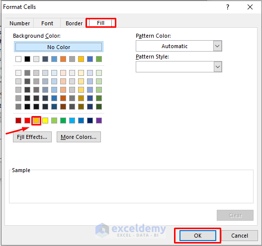
- Select Fill in the header tab.
- Select a color.
- Click OK.
- Click OK in the New Formatting Rule dialogue box.
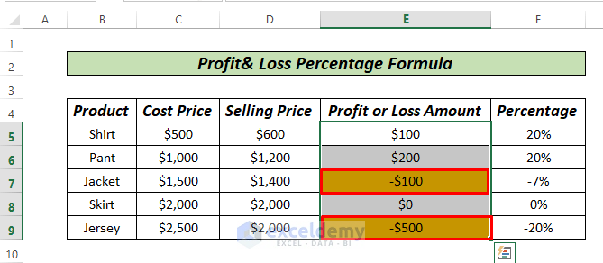
Our result will look like the following image.
Method 4 – Profit and Loss Percentage Formula along with IF Function
STEPS:
- In cell E5 enter the following formula:
=IF(D5=C5,"No profit,No loss",IF(D5<C5,"Loss",IF(D5>C5,"Profit")))
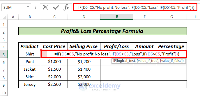
The IF function will return No Profit No Loss when Cost Price equals Selling Price, Profit when Cost Price is less than Selling Price, and Loss when Cost Price is greater than Selling Price.
- Press ENTER.
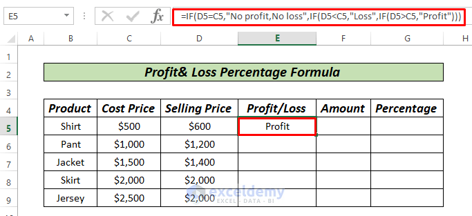 Drag the formula down using the right click button on the mouse to AutoFill the rest of the series.
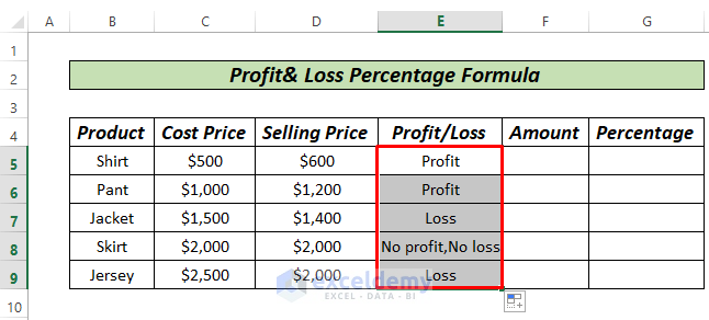 Follow Method 1.
As a result, our data set will look like the following image.
Download Practice Workbook
<< Go Back to Formula List | Learn Excel
Get FREE Advanced Excel Exercises with Solutions!

Nice
Hello Vijay,
Thanks for your appreciation.
Regards
ExcelDemy