How to Merge Duplicates in Excel (6 Ways)

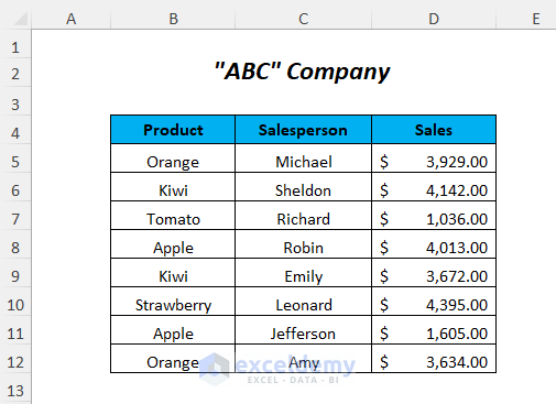
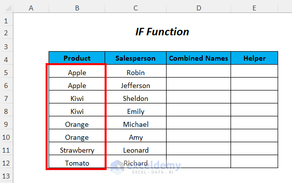
We’ll use the following table to demonstrate how to merge duplicates in Excel.

Method 1 – Using the IF Function to Merge Duplicates with Text

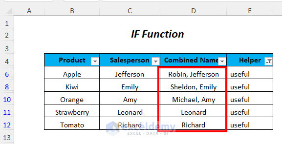
We will combine the Salesperson’s names for the duplicate products.

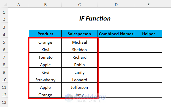
• We have added two columns, Combined Names and Helper.
• Select the data range
• Go to the Home tab, select Sort & Filter and choose Custom Sort.

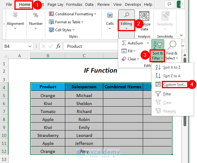
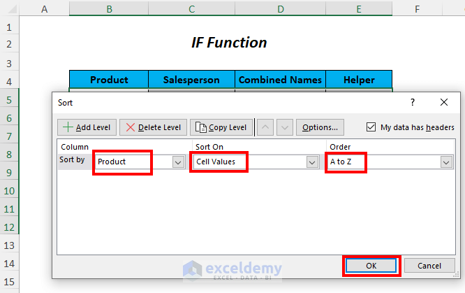
• The Sort dialog box will open.
• Select the following:

Sort by → Product
Sort On → Cell Values
Order → A to Z

• Press OK.

• This will sort the names of the products from A to Z.

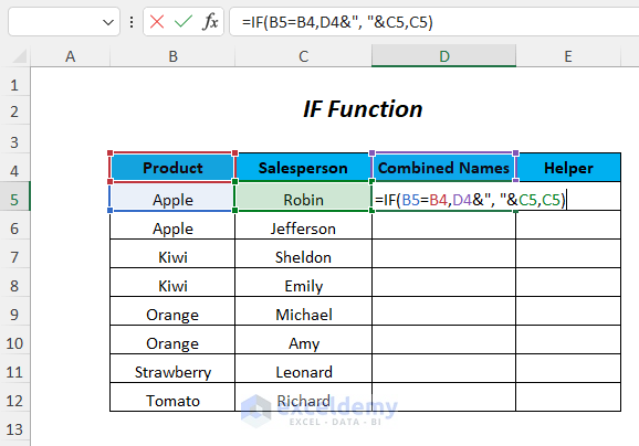
• Use the following formula in cell D5.

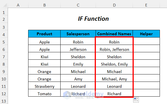
• Hit Enter and drag down the Fill Handle tool.

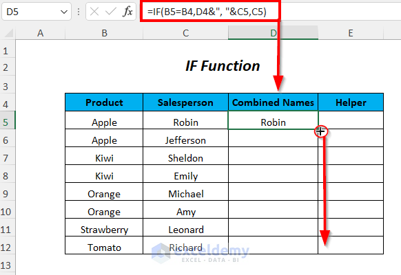
• This combines the names of the Salesperson for the duplicate rows.

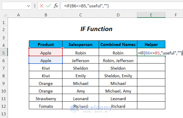
• Use the following formula in cell E5.

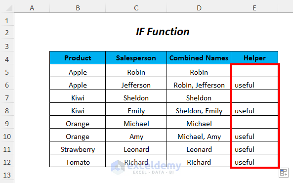
• Hit Enter and drag down the Fill Handle.

• You will get useful for the duplicate rows.

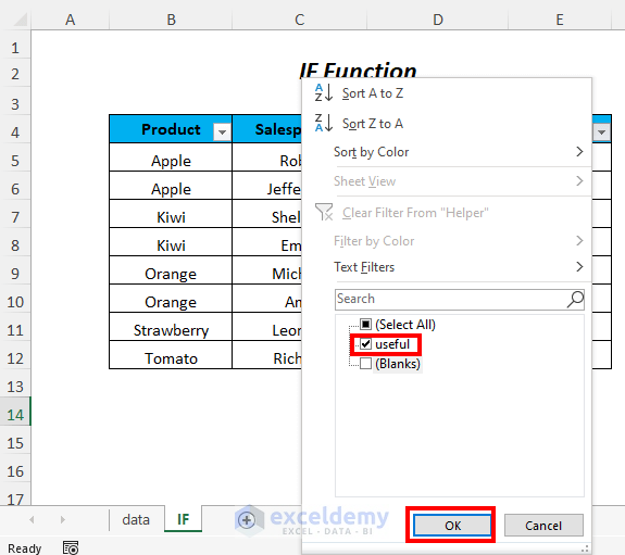
• Select the data range.
• From Sort & Filter, choose Filter.

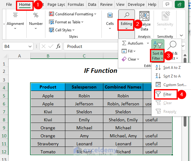
• The filter signs will appear in every column of the table.
• Select the drop-down of the Helper column.

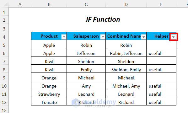
• Choose the useful option and click OK.

Result:

Method 2 – Using the Merge & Center Option to Merge Duplicates in Excel

We’ll merge the cells in the Product column that have the same values.

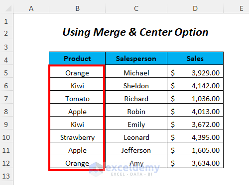
• Follow the Steps of Method 1 to sort the product names from A to Z.
  
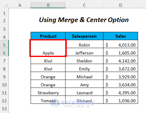
• Select the two cells containing Apple.
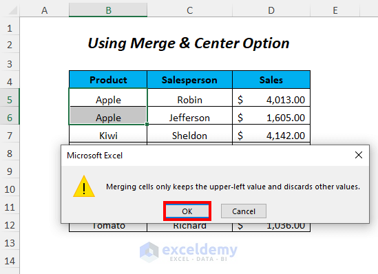
• Go to the Home tab and click on Merge & Center.

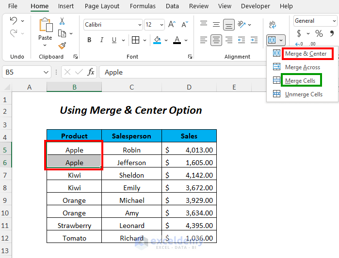
• You’ll get a message box. Press OK.

• This merges the first two cells containing Apple.

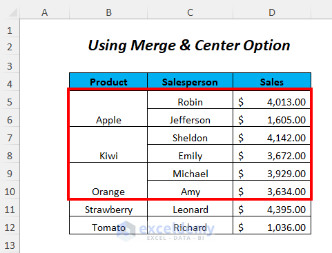
• Repeat for other duplicate cells to get the following table.

Method 3 – Using Power Query 

We’ll merge the duplicate rows in the Product column.

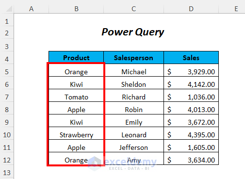
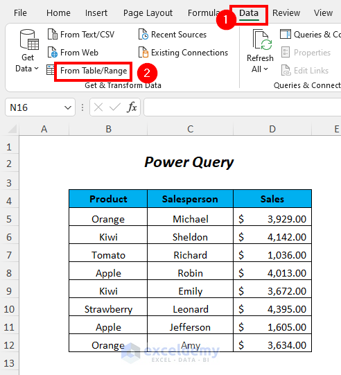
• Go to the Data tab and select From Table/Range.

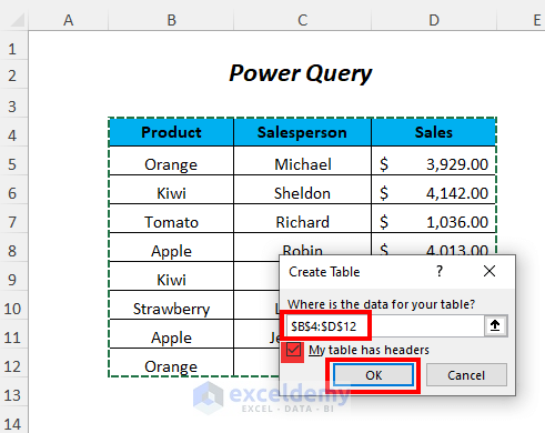
• The Create Table dialog box will open.
• Select the data range.
• Check My table has headers and press OK.

• A Power Query Editor will appear

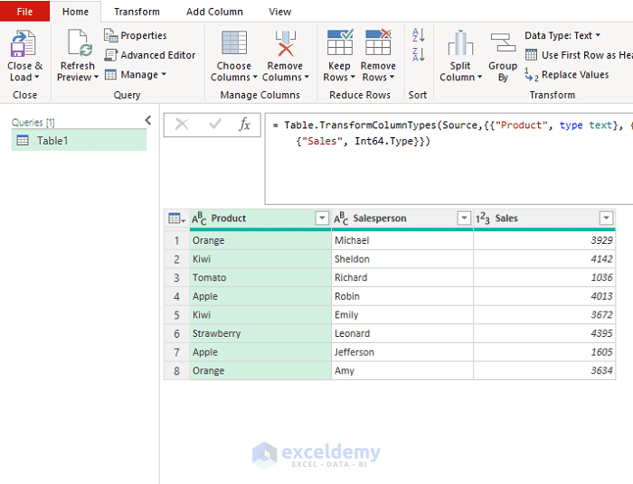
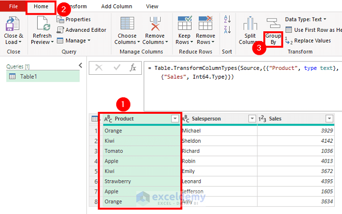
• Select the Product column where you have duplicate values.
• Go to Home and select Group By.

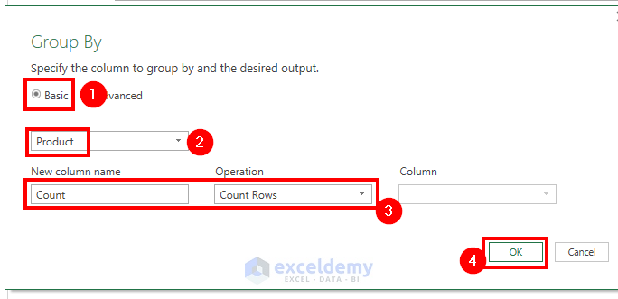
• The Group By wizard will pop up.
  Select the following options:

Basic
Product (the name of the column)
New column name → Count
Operation → Count Rows

• Press OK.

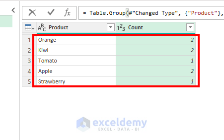
Result:

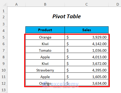
Method 4 – Using a Pivot Table to Merge Duplicates in Excel

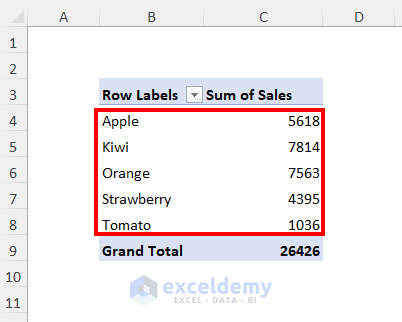
We’ll merge the duplicate rows in Product and sum up their corresponding Sales values.

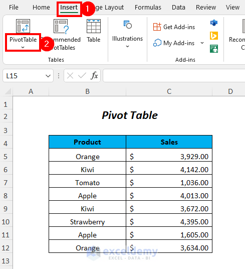
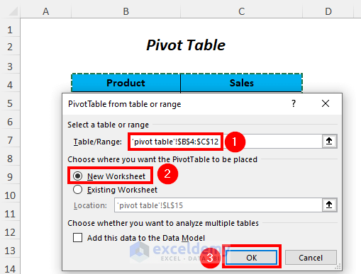
• Go to Insert and select PivotTable.

• The PivotTable from table or range dialog box will open.
• Select the data range.
• Check New Worksheet and press OK.

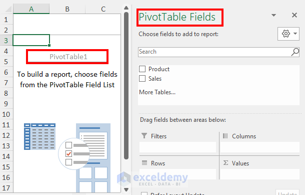
• A new sheet will appear where you have two panels, PivotTable1 on the left side and PivotTable Fields on the right side.

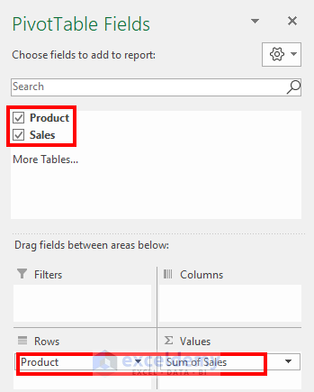
• Drag Product to the Rows area and Sales to the Values area.

Result:

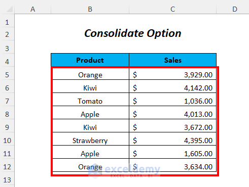
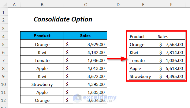
Method 5 – Using the Consolidate Option to Merge Duplicates in Excel

We’ll merge the duplicate rows and sum up their corresponding Sales values.

Steps:

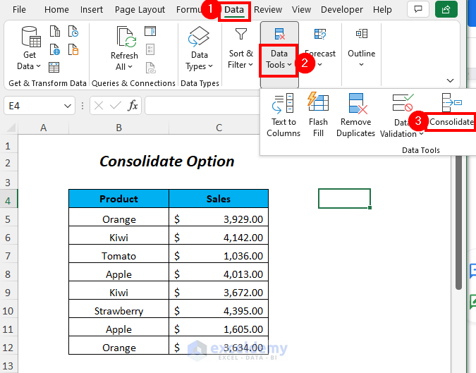
• Select the cell where you want to get the output.
• Go to Data and select Consolidate.

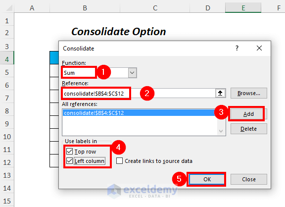
• The Consolidate wizard will open.
• Select Sum (or any other function) as Function, data range as Reference, and click on Add.
  
• Check the Top row and Left column options and press OK.

• You will get the merged values in your selected area.

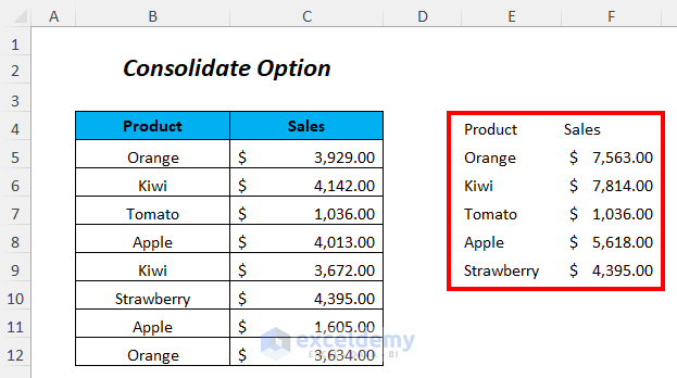
• We have used borders for the new consolidated table.

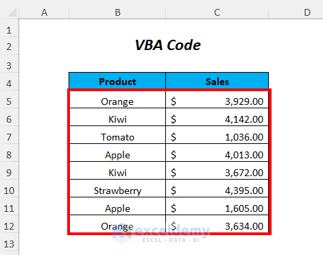
Method 6 – Using VBA Code to Merge Duplicates in Excel

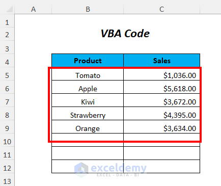
We’ll merge the duplicate rows and sum up their corresponding Sales values.

• Go to the Developer tab and select Visual Basic.

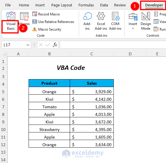
• The Visual Basic Editor will open up.
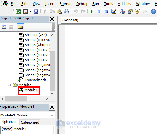
• Go to Insert and select Module.

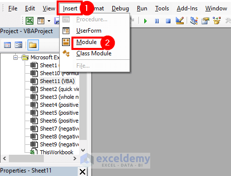
• A Module will be created.

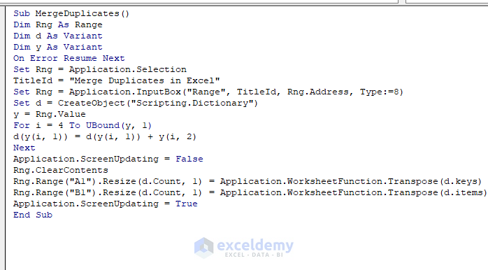
• Insert the following code.

Sub MergeDuplicates()

Dim Rng As Range
Dim d As Variant
Dim y As Variant

On Error Resume Next

Set Rng = Application.Selection
TitleId = "Merge Duplicates in Excel"
Set Rng = Application.InputBox("Range", TitleId, Rng.Address, Type:=8)
Set d = CreateObject("Scripting.Dictionary")
y = Rng.Value

For i = 4 To UBound(y, 1)

d(y(i, 1)) = d(y(i, 1)) + y(i, 2)

Next

Application.ScreenUpdating = False

Rng.ClearContents
Rng.Range("A1").Resize(d.Count, 1) = Application.WorksheetFunction.Transpose(d.keys)
Rng.Range("B1").Resize(d.Count, 1) = Application.WorksheetFunction.Transpose(d.items)

Application.ScreenUpdating = True

End Sub

We have declared Rng as Range and d, y as Variant and used On Error Resume Next to ignore the error and continue or resume the code execution to the next cell.

The FOR loop is used for a range of rows starting from i = 4 (as our data table started from row number 4) and the UBOUND function will determine the size of the array.

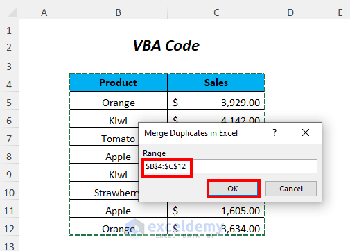
• Press F5
• The Merge Duplicates in Excel (the name of the custom function) wizard will open.
• Select the range and press OK.

Result:

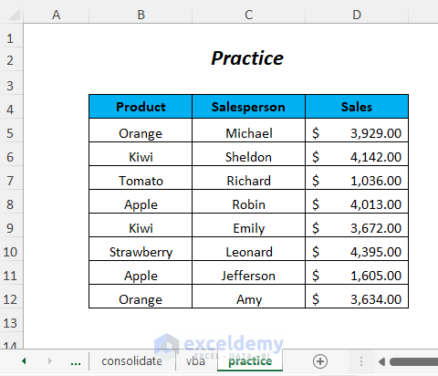
Practice Section

We have provided a Practice section like below in a sheet named Practice so you can test these methods.

Download the Practice Workbook

Merge Duplicates in Excel: Knowledge Hub

• Merge Duplicate Rows in Excel
• Combine Duplicate Rows in Excel without Losing Data
• How to Combine Duplicate Rows and Sum the Values in Excel

<< Go Back to Learn Excel