How to Merge Duplicate Rows in Excel (3 Methods)

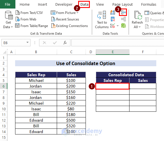
Method 1 – Using the Consolidate Command

Steps:

• Select a blank cell.
• Go to the Data tab > Data Tools group > Consolidate.
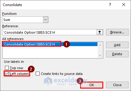
  The Consolidate dialog box appears.
• In the Consolidate dialog box:
  • Select Sum in the Function drop-down. Or any other option useful for your task.
  • Choose the range in the Reference box. Your selected range will appear inside the “All references” box.
  • Check the Left column and click OK.

  

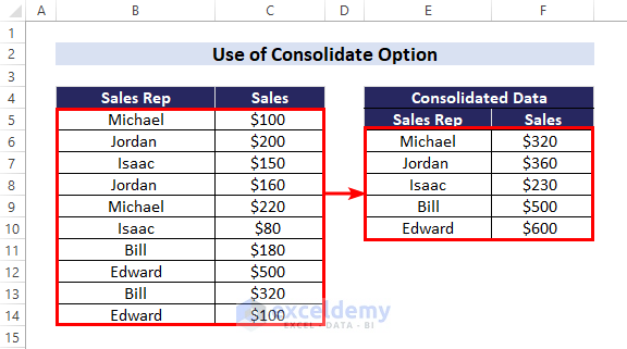
You will get the unique rows from your initial data.

Read More: How to Combine Duplicate Rows in Excel without Losing Data

Method 2 – Applying the Subtotal Feature

Steps:

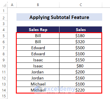
• Select your data.
• Go to the Home tab > Editing group > Sort & Filter dropdown > Sort A to Z.
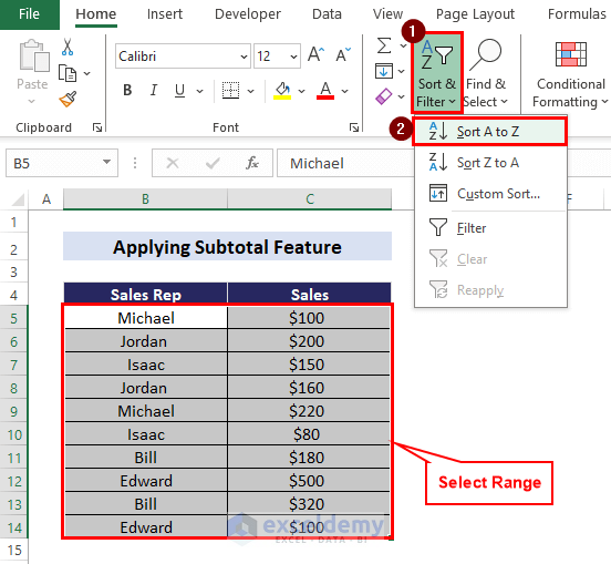  The sales values with their corresponding representatives have been arranged in the following order.
  
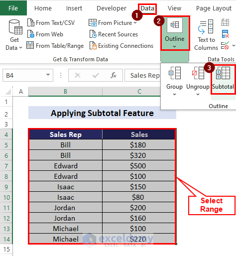
• Select your data again.
• Go to Data tab > Outline drop-down > Subtotal.
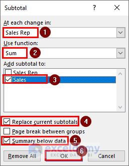
  The Subtotal dialog box will appear.
• In the Subtotal dialog box:
  • Select the first column name in the “At each change in” field.
  • Select Sum in the “Use function” field.
  • Select the 2nd column name from the “Add subtotal to” menu.
  • Mark the “Replace current subtotals” and “Summary below data” checkboxes.
  • Press OK.

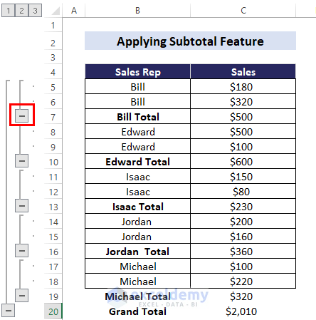
  The sales for each representative will be grouped, and their sales values will be added up.

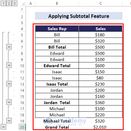
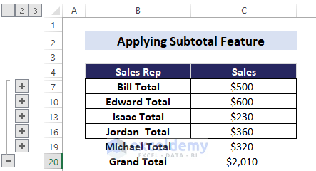
• Click on the minus(-) sign to collapse the Subtotal groups.
  

Here is the final result.

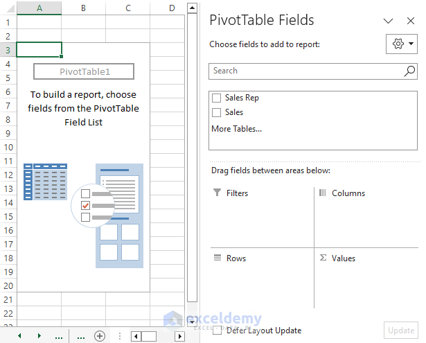
Method 3 – Using the Pivot Table Feature

Steps:

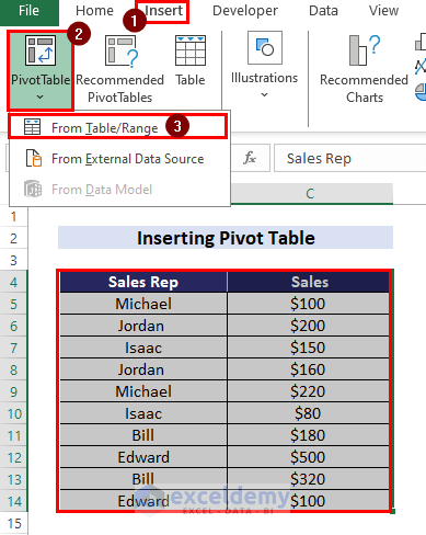
• Select your data > Insert tab > PivotTable drop-down > From Table/Range.
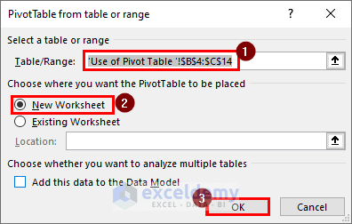
  The “PivotTable from table or range” dialog box will open up.
• From the “PivotTable from table or range” dialog box:
  • Click on the New Worksheet button. Or, select the Existing Worksheet.
  • Press OK.

  You will be taken to a new sheet, where the PivotTable and PivotTable Fields will appear on the left and right sides.
  

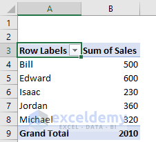
• Drag down the Sales Rep to the Rows area and Sales to the Values area.
  

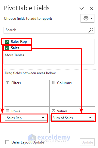
The PivotTable will appear on the left side, and you can see the combined data with their corresponding unique values.

Read More: Combine Duplicate Rows and Sum the Values in Excel

Download the Practice Workbook

<< Go Back to Merge Duplicates in Excel | Learn Excel