How to Combine Duplicate Rows and Sum the Values in Excel: 4 Suitable Ways

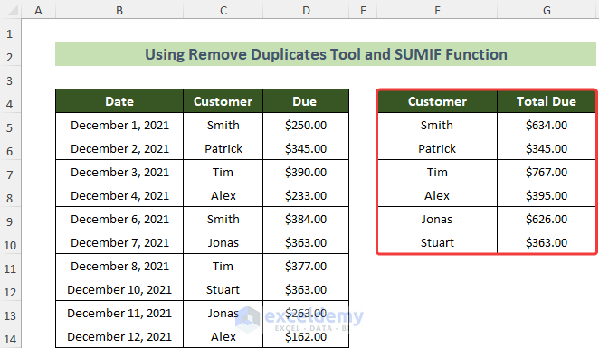
Method 1 – Using Remove Duplicates Tool and SUMIF Function

Steps:

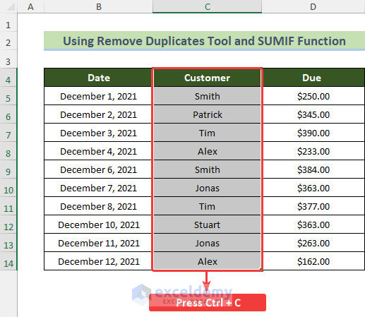
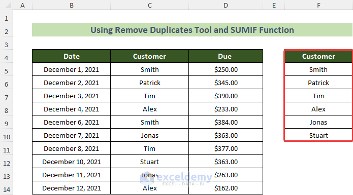
• Copy the Customer column (make sure you start copying from the header Customer) using CTRL+C or from the ribbon.

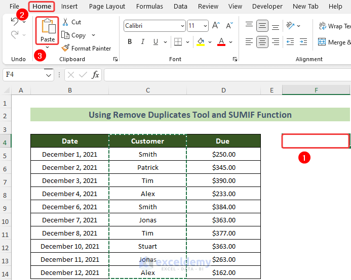
• Select any cell where you want to paste it (cell F4 here) >> go to the Home tab >> click on Paste button.

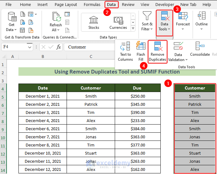
• While selecting the copied cells, go to Data Tab >> Data Tools group >> Remove Duplicates tool.

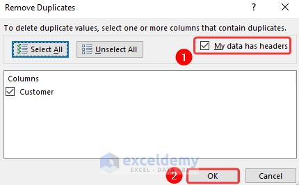
• The Remove Duplicates dialogue box will appear. Make sure to mark My data has headers tick box. Select the listed columns (in our case, Customer) and then press OK.

• The duplicates have been removed.

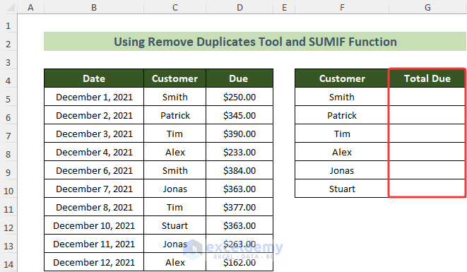
• Make a new header beside Customer naming it Total Due for sum.

• Select cell G5 underneath the new header and write the following function using SUMIF function.

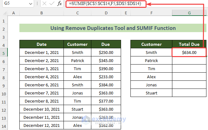
Refers to calculating the summation value of F5 according to the data in D$5:D$14 corresponding to the names in the range of C$5:C$14. You can adjust the formula accordingly.

• Copy this formula to the next few cells by dragging the fill handle below up to the cell where the column of Customer ends.

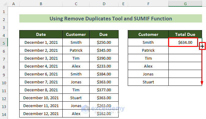
The formula will be copied to all the cells below and you will be able to sum the values of your duplicate rows in Excel.

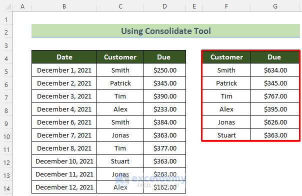
Method 2 – Using Consolidate Tool to Combine Duplicate Rows and Sum the Values

Steps:

• Copy and paste the headers from the preliminary data in the desired location.

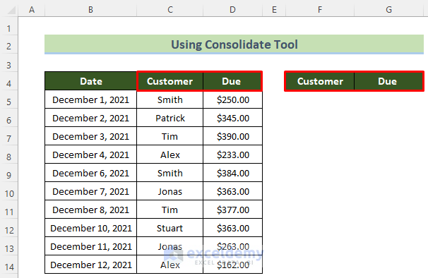
• Select the cell below the first copied header.
• Go to the Data Tab >>  Data Tools group >> Consolidate tool.

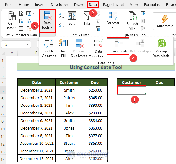
• The Consolidate dialogue box will appear. In the Function: dropdown box select Sum (it should already be there). Mark the Left Column tick box.
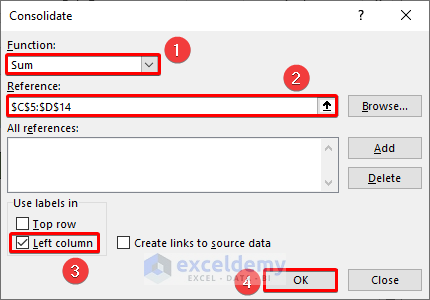
• Click into the Reference box and using a mouse select the cells without headers (it is very important that you do that) or you can manually input cells range (don’t forget to use $ to make cells absolute – i.e. in our example it is $C$5:$D$14. You know what? Use a mouse, that way excel will input it automatically). Click OK.

Get your sum values in Excel successfully with combined duplicate rows.

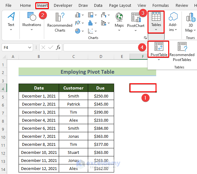
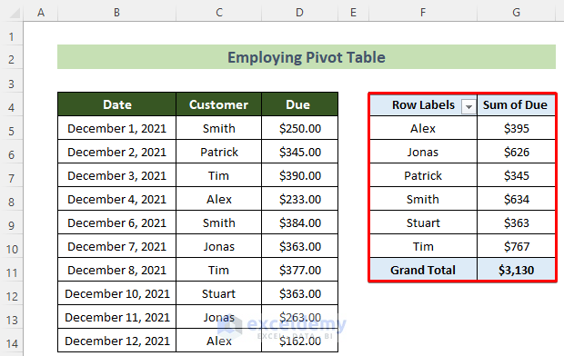
Method 3 – Employing Pivot Table Feature

Steps:

• Select an empty cell where we will make a Pivot Table.
• Go to the Insert tab >> Tables group >> Pivot Table tool.

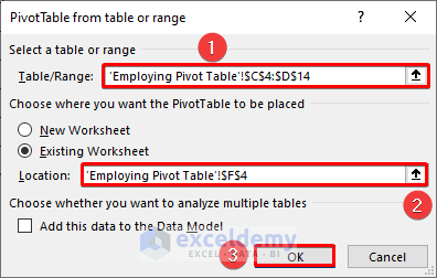
• The PivotTable from table or range dialogue box will appear. For the data to analyze in the Table/Range: text box, select the range with a mouse just like Consolidation but with headers. This time in the box a new term for sheet name will also show up as pivot table can be used to get data from different worksheets too. Like in our example it is ‘Employing Pivot Table’!$C$4:$D$14 for selecting cells C4 to D14 in the Employing Pivot Table sheet.
• To input to a cell in the current worksheet select Existing Worksheet and in the location select a cell with the mouse or write ‘Worksheet Name’!Cell Id. Make sure you make the cell absolute. It is ‘Employing Pivot Table’!$F$4 for inputting the value at cell F4 in the Employing Pivot Table worksheet. Click on OK.

• A pivot table is created.
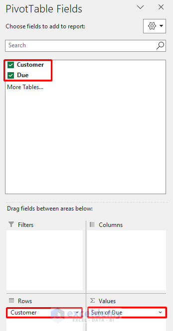
• Go to the PivotTable Fields pane on the right.
• Drag to put the Customer field into the Rows area and Sum of Due into the Values area.

Get the Sum of dues of all customers with their names in a Pivot Table.

Method 4 – Applying VBA Code to Combine Duplicate Rows and Sum Values

Steps:

• Go to the Developer tab >> Visual Basic tool.

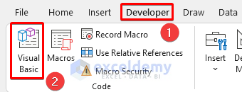
• The VB Editor window will open.
• Go to the Insert tab >> Module option.

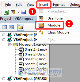
• A new module named Module1 will be created.
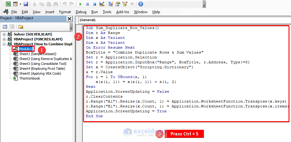
• Double-click on Module1 and write the following code in the code window.

Sub Sum_Duplicate_Row_Values()
Dim r As Range
Dim x As Variant
Dim a As Variant
On Error Resume Next
BoxTitle = "Combine Duplicate Rows & Sum Values"
Set r = Application.Selection
Set r = Application.InputBox("Range", BoxTitle, r.Address, Type:=8)
Set x = CreateObject("Scripting.Dictionary")
a = r.Value
For i = 1 To UBound(a, 1)
    x(a(i, 1)) = x(a(i, 1)) + a(i, 2)
Next
Application.ScreenUpdating = False
r.ClearContents
r.Range("A1").Resize(x.Count, 1) = Application.WorksheetFunction.Transpose(x.keys)
r.Range("B1").Resize(x.Count, 1) = Application.WorksheetFunction.Transpose(x.items)
Application.ScreenUpdating = True
End Sub

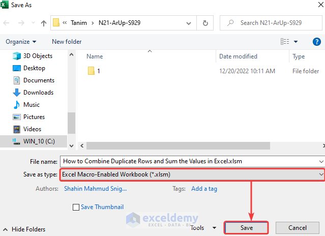
• Press Ctrl + S.

• A Microsoft Excel dialogue box will appear.
• Click on the No button.

• The Save As dialogue box will appear.
• Choose the Save as type: option as .xlsm file and click on the Save button.

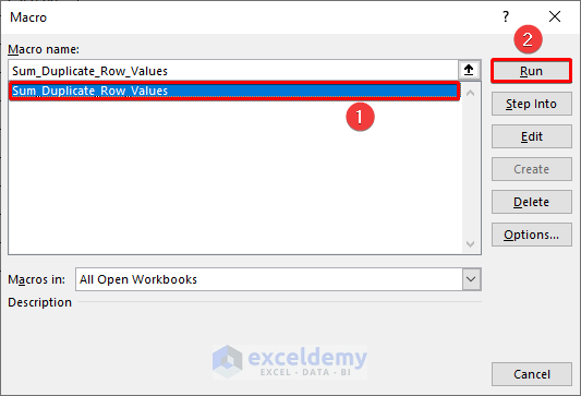
• Close the VB Editor and go to the Developer tab >> Macros tool.

• The Macro window will appear.
• Choose the Sum_Duplicate_Row_Values macro and click on the Run button.

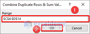
• The created Combine Duplicate Rows & Sum Values dialogue box will appear.
• Refer to the cells C4:D14 in the Range text box and click the OK button.

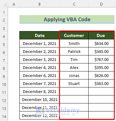
Get your desired result in the existing columns.

Download Practice Workbook

You can download our practice workbook from here for free!

Further Readings

• Merge Duplicate Rows in Excel
• How to Combine Duplicate Rows in Excel without Losing Data

<< Go Back to Merge Duplicates in Excel | Learn Excel