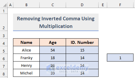
Method 1 – Remove Inverted Commas in Excel Using a Multiplication
Steps:
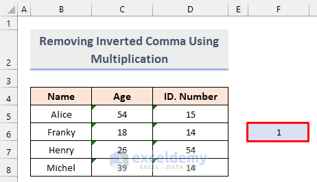
- Enter 1 in any random cell in the worksheet and copy the cell by pressing Ctrl+C.
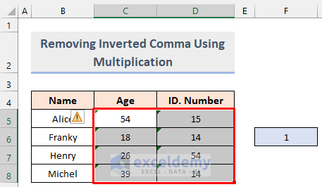
- Select the entire cell range containing inverted commas.
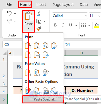
- Go to the Home tab and select Paste Special.
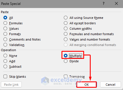
- Select Multiply and click OK.
- Since the values are multiplied by 1, they will be without the inverted commas:
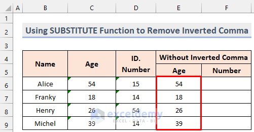
Method 2 – Using the SUBSTITUTE Function to Remove Inverted Commas
Steps:
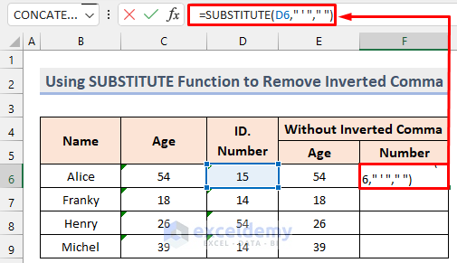
- Create separate columns to store the removed data. Select one cell in those columns and enter the following formula in the formula bar.
=SUBSTITUTE(C6," ' "," ")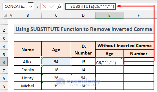
In the formula, data is imported from C6. It assigns a sign/letter/number to replace and the destination cells for the replaced data.
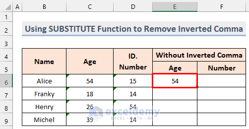
- Press Enter to see the output.
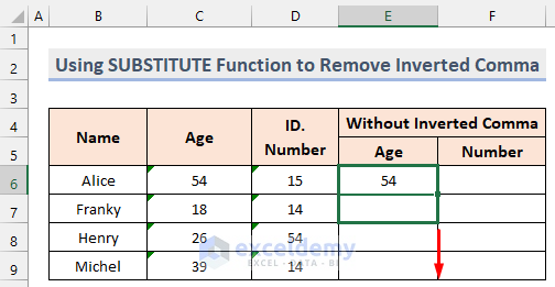
- Drag down the Fill Handle to see the result in the rest of the cells.
The final output is:
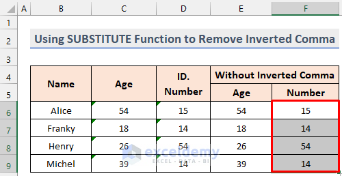
- Select F6, enter the following formula in the formula bar and press Enter.
=SUBSTITUTE(D6," ' "," ")
Data in D6 has no inverted commas.
- Drag down the Fill Handle to see the result in the rest of the cells.
Read More: How to Remove Comma in Excel Using Formula
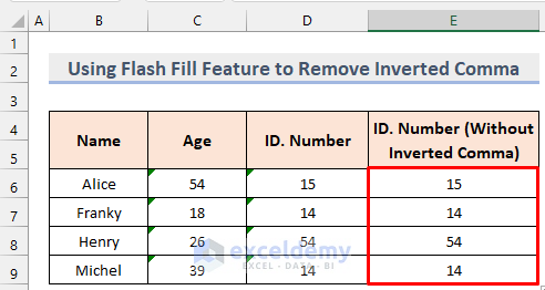
Method 3- Using the Flash Fill Feature to Remove Inverted Commas
Steps:
- Create a new column adjacent to the column containing data with inverted commas.
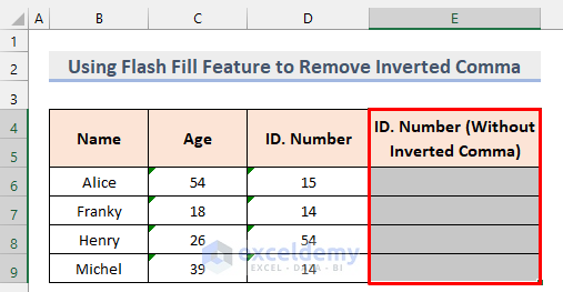
- Select the first adjacent cell in the new column and enter the same data without inverted commas.
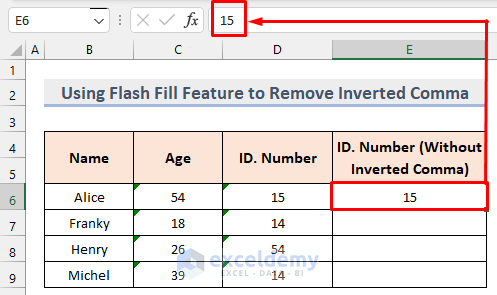
- Press Enter to see the output.
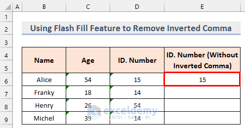
- Select the cell.
- Drag down the Fill Handle to see the result in the rest of the cells.
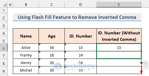
This is the output.

- Select the tiny box at the end of the Fill Handle box and select Flash Fill.
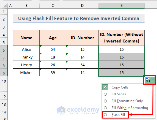
This is the final output.
Method 4- Using the LEFT and LEN Functions
Steps:
- Create a new column to store the data without inverted commas. Select the first cell and enter the following formula in the formula bar.
=LEFT(C6,LEN(C6))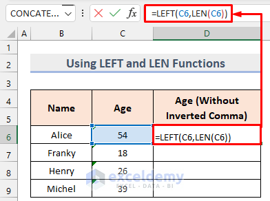
The LEFT function is used because the inverted commas were on the left. The LEN function indicates the length of the string, but avoids the inverted comma and takes the value only.
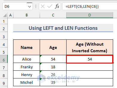
- Press Enter to see the data without inverted commas.
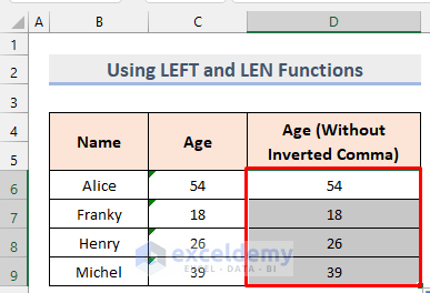
- Drag down the Fill Handle to see the result in the rest of the cells.
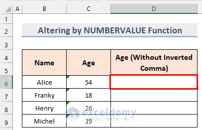
Method 5- Applying the NUMBERVALUE Function
Steps:
- Select the target cell to get the new value:
- Enter the following code in the formula bar and press Enter.
=NUMBERVALUE(C6)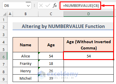
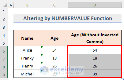
- Drag down the Fill Handle to see the result in the rest of the cells.
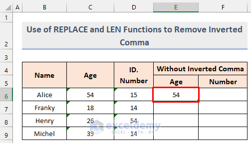
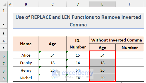
Method 6- Using the REPLACE and LEN Functions to Remove Inverted Commas
Steps:
- Select a new cell to get the data without inverted commas and enter the following code in the formula bar.
=REPLACE(C6,LEN(C6)+1,LEN(C6),"")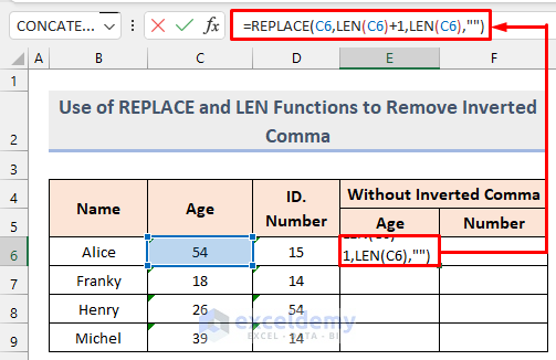
- Data in C6 is displayed without inverted commas in the new cell:
- Drag down the Fill Handle to see the result in the rest of the cells.
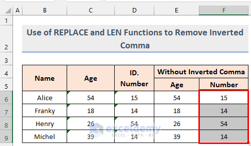
- For the ID. Number column, you can do the same, changing the formula:
=REPLACE(D6,LEN(D6)+1,LEN(D6),"")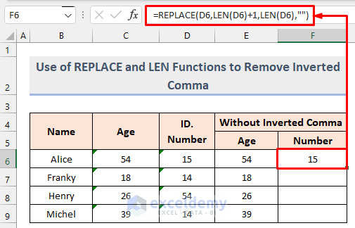
- Drag down the Fill Handle to see the result in the rest of the cells.
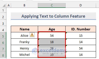
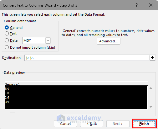
Method 7- Applying the Text to Column Feature
Steps:
- Select a column containing the data with inverted commas.
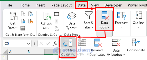
- Go to the Data tab.
- Select Text to Columns in Data Tools.
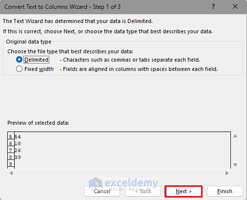
- In the dialog box, click Next.
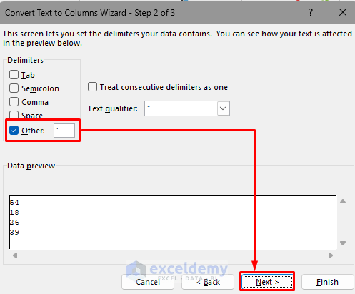
- Click Other and enter (‘) in the box.
- Click Next.
- Click Finish.
This is the output.
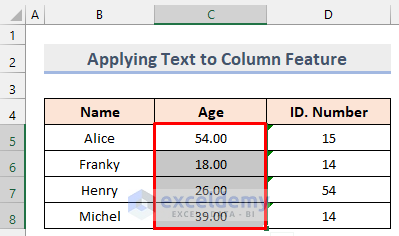
- Repeat the process for the other column.
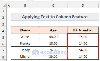
This is the output.
Things to Remember
- The SUBSTITUTE function replaces all the inverted commas with a blank space.
- Applying the Text to Column feature will convert all numeric values to numbers, date values to date, and all other formats to text.
Download Practice Workbook
Download the practice workbook.
Related Articles
- How to Change Comma Separator in Excel
- How to Remove Commas in Excel from CSV File
- How to Remove Comma from Currency in Excel
<< Go Back To Remove Comma in Excel | Data Cleaning in Excel | Learn Excel
Get FREE Advanced Excel Exercises with Solutions!
