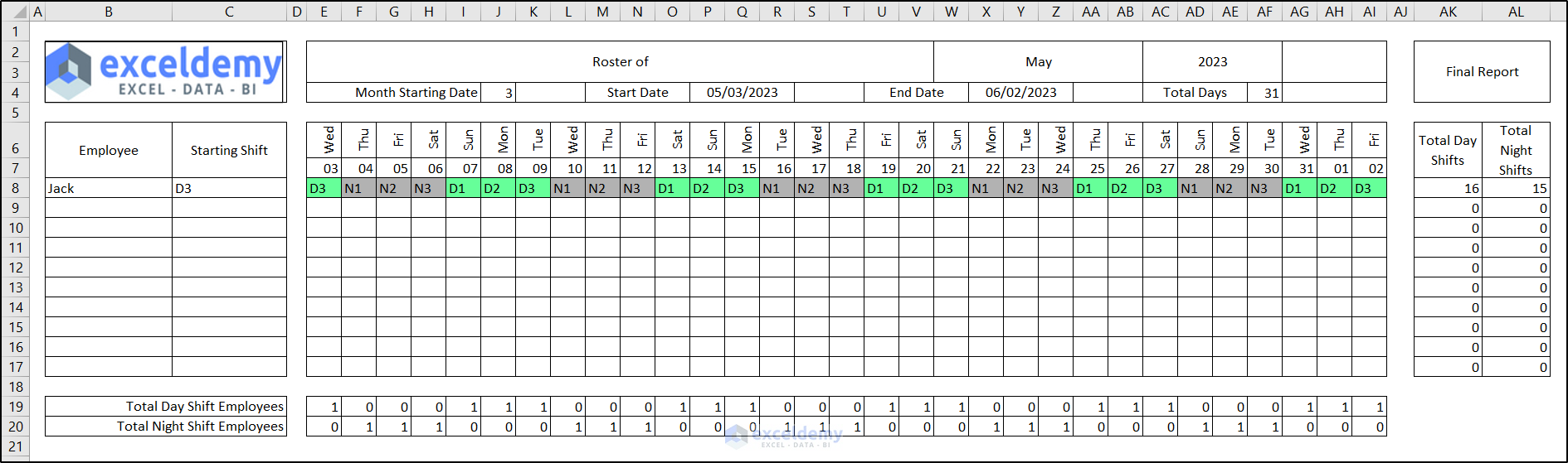
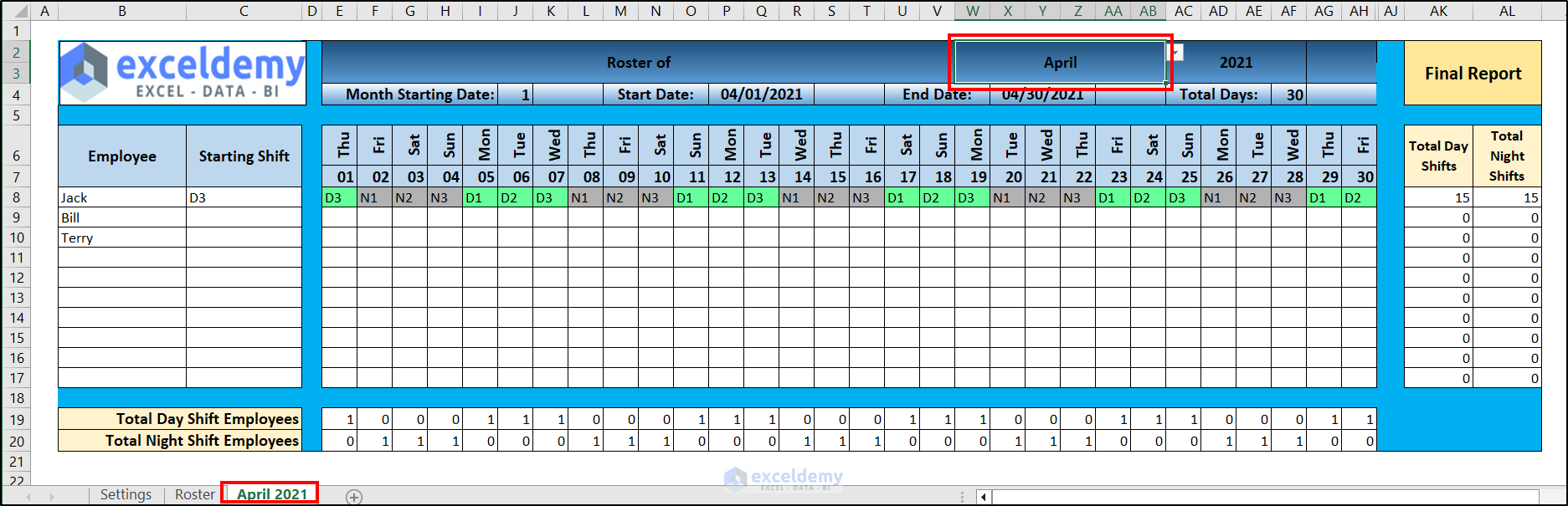
Here’s a roster template that we will be making throughout this article. You can follow along and make changes if you want a modified version, or simply download the template worksheet and use it as-is.
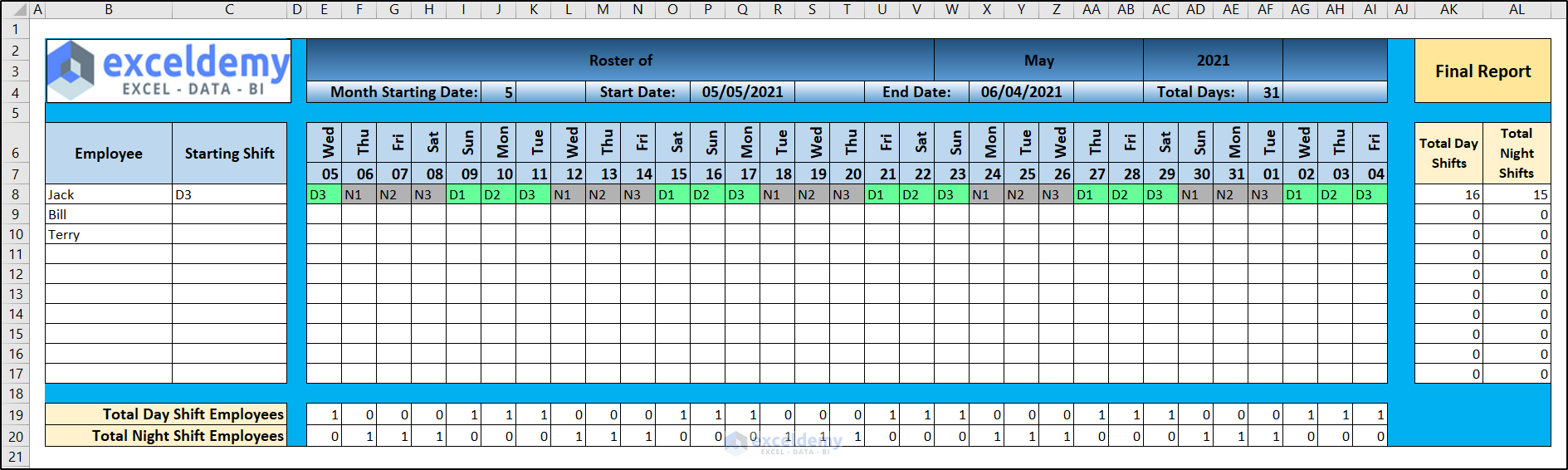
How to Make a Roster in Excel: Step-by-Step Guide
Step 1 – Create a Spreadsheet for Different Attributes
You need a spreadsheet that contains all the repeatable information like employee names and months. This sheet is also important to manipulate data throughout the workbook. It is the basis of using the workbook as a template.
We have included months, years, weekends, shift types, shift codes, and employee names in different columns.
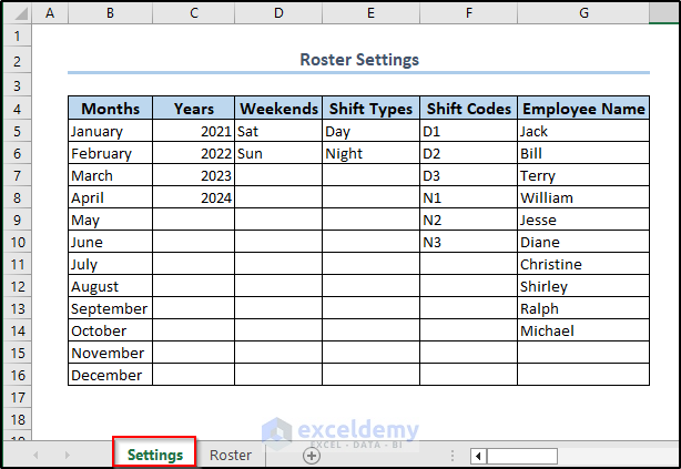
We have named the sheet “Settings” which will be helpful in later steps. Be careful with the name you will pick here as some steps will change accordingly when you need to input it.
Step 2 – Make Named Ranges for Particulars
This is the basis of all the dynamic operations of the roster. We are going to name each range so that we can use recall them in formulas. We have used dynamic ranges except for the months and weekends as the roster can then work for new entries, such as years, employees, or shift types.
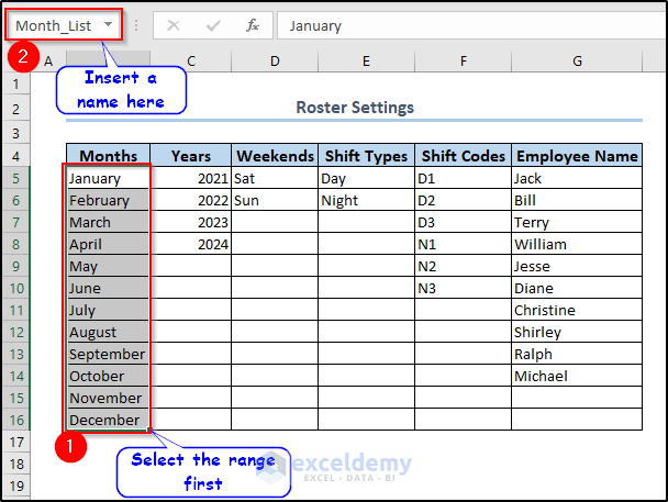
- To name a static range, select the range and insert a name in the Name Box.
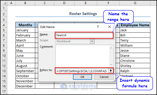
- To name a range dynamically, go to the Formulas tab, select Name Manager from the Defined Names group and select New from the Name Manager box.
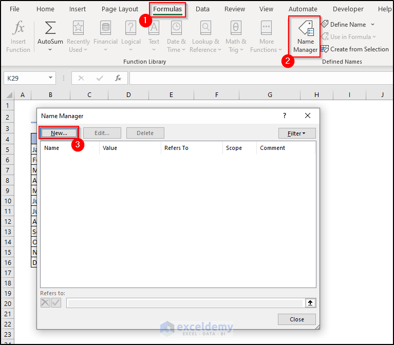
- In the next Edit Name box, name the range beside the Name field and insert formulas (see below) that define the dynamic range beside the Refers to field.
- After clicking OK and closing all of the boxes, you will have the named ranges.
We have to define each dynamic or static range individually. The formulas we have used for each range are:
Employee_List (employee names):
=OFFSET(Settings!$G$4,1,0,COUNTA(Settings!$G:$G)-1,1)Shift_Codes (Shift Codes):
=OFFSET(Settings!$F$4,1,0,COUNTA(Settings!$F:$F)-1,1)YearList (Years):
=OFFSET(Settings!$C$4,1,0,COUNTA(Settings!$C:$C)-1,1)
Formula Explanation
OFFSET(Settings!$G$4,1,0,COUNTA(Settings!$G:$G)-1,1)
The COUNTA function counts the number of cells in the range within it. The Settings! before the range is from the spreadsheet name.
COUNTA(Settings!$C:$C)-1 is the height argument of the OFFSET function while cell G4 is the reference. The OFFSET function basically picks up the range below the G4 cell and automatically puts it in the range “YearList”.
Step 3 – Resize Cells for Master Sheet
- Merge B2:C4 to hold a place for the logo.
![]()
- Merge E4:V3 to hold the title, W2:AB3 to hold the monthly value, AC2:AF3 to place the year, and AG2:AI3 to keep up with the roster below (we are keeping places for all days of a month in it).

- Merge E4:I4, K4:L4, M4:O4, P4:R4, S4:T4, U4:W4, X4:Z4, AA4:AB4, AC4:AE4, and AG4:AI4 and prepare the headers like follows.

Step 4 – Insert Logo and Headers
Insert the company logo and headers next, in the prepared cells.
These are the headers and the logo we have selected to put in our template.
![]()
You can modify these on your own but for beginners, we recommend just following them as the steps suggest.
Step 5 – Prepare Cells for Month and Year
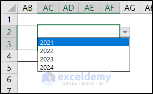
We will assign drop-down menus to select months and years.
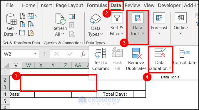
- Select cell W2 and select Data Validation from the Data Tools group of the Data tab.
- In the Data Validation box, select List under Allow.
- Clicking on Source field and press F3 on your keyboard. Select the named range for months from the “Settings” sheet.
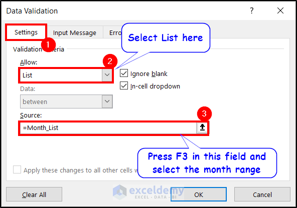
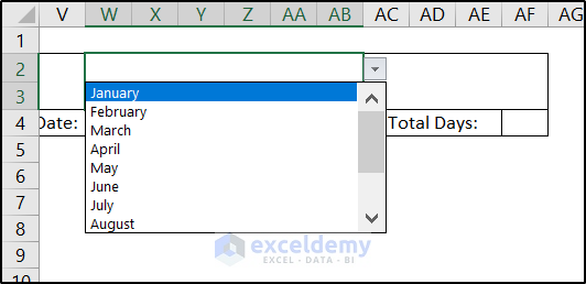
- Clicking on OK and there will be a drop-down list available in the cell, with all the month names in it.
- Follow similar steps for the cell next it for the year values.
- Select random values for them and in cell J4 that will help us with the formulas for the next portions.

Step 6 – Prepare Cells for Other Month Particulars
- In cell P4, copy the following formula:
=IFERROR(DATEVALUE(J4&W2&AC2),"")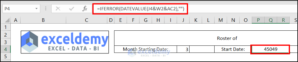
Formula Explanation
- J4&W2&AC2 puts together the values of these three cells to make up a date.
- DATEVALUE(J4&W2&AC2) converts them into Excel’s date value.
- We have put the previous function in an IFERROR function so that in cases of error (such as values like 32 in cell J4), Excel doesn’t display any error message.
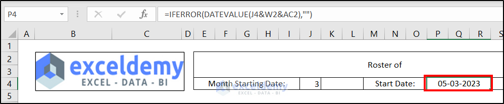
- You may have noticed the date is not in the correct format. To put it in the proper format, select the cell and press Ctrl+1 on your keyboard.
- This will open up the Format Cells.
- Go to the Number tab, select Custom under Category, and put a custom mm-dd-yyyy format on the right.
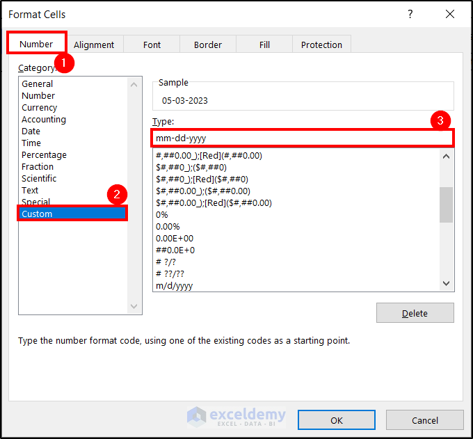
- Click on OK.
- In cell X4, insert the following formula and use the same formatting technique:
=IFERROR(EOMONTH(P4,0)+J4-1,"")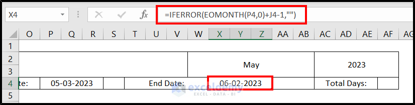
Formula Explanation
IFERROR(EOMONTH(P4,0)+J4-1,””)
EOMONTH(P4,0) indicates the month-ending value of the date in cell P4. We have used the argument 0 so that it returns the end value of the month in cell P4.
The value after that (+J4-1) is there to make sure it is exactly a month after P4 in case the starting date is not the first day of the month and disregards how many days the month has.
We put that inside an IFERROR function so that it doesn’t display an error value in case of invalid input such as more than 31 days as the starting day.
- To count the “Total Days”, we have put the following formula in cell AF4.
=X4-P4+1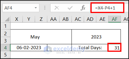
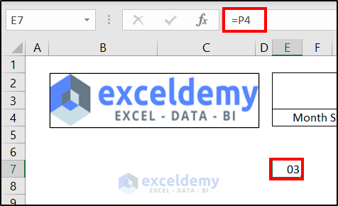
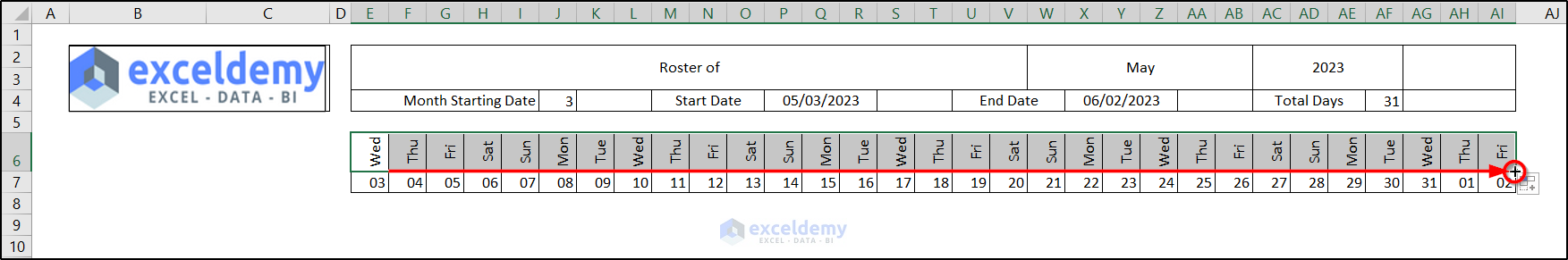
Step 7 – Insert Dynamic Dates and Days
Our roster will have both days and dates above all the assigned shifts.
- Put this function inside cell E7 so that it maintains the starting date. We are using the dd format as we don’t want the cells to be too large for this.
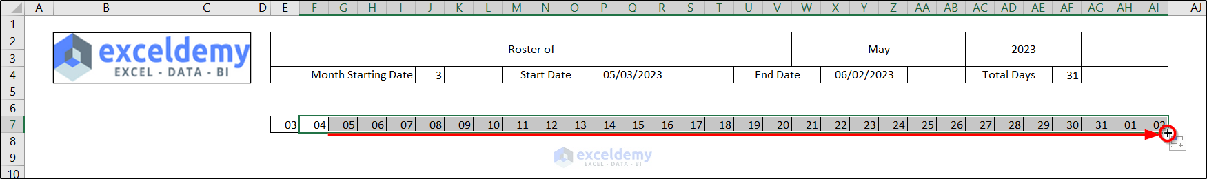
- In cell F7, copy the following formula and use the format dd:
=IF(E7>=$X$4,"",E7+1)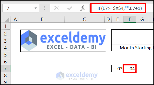
- Replicate the formula until cell AI7 via the Fill Handle.
- In cell E6, copy the following formula for the day:
=TEXT(E7,"ddd")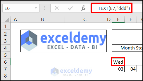
- We have also changed the alignment vertically. To do that, press Ctrl+1 while the cell is selected and use 90 degrees in the Alignment tab of the Format Cells box that will open up.
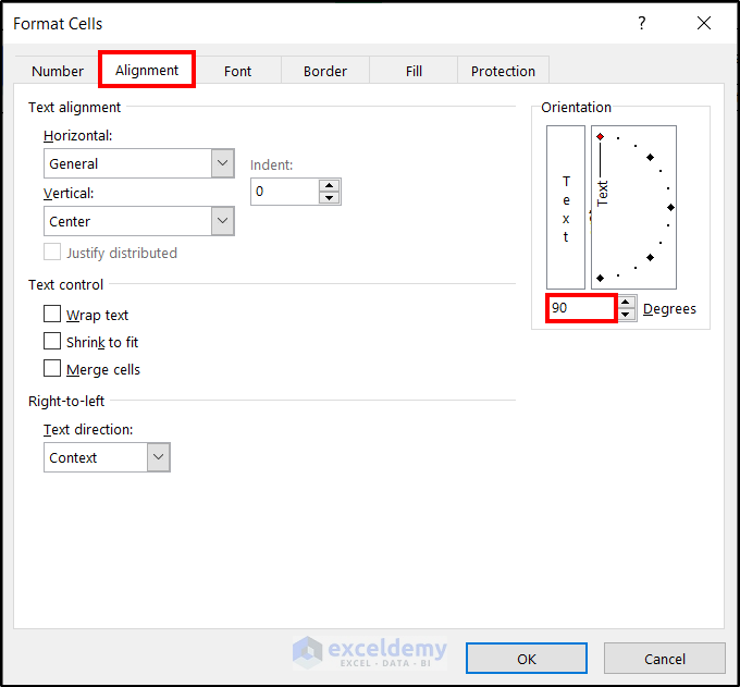
- After pressing OK, the day will look like this now.
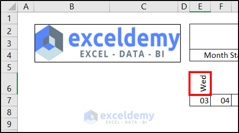
- Drag the fill handle icon to cell AI6 to replicate the formula.
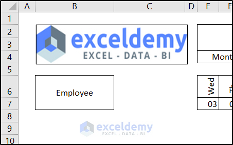
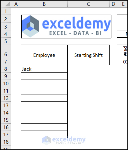
Step 8 – Organize Employee Sheet Columns Dynamically
The employee list exists in the “Settings” sheet. We need to modify the employee column in the roster so it imports the value from that list and an ex-employee or a new one can be edited from there and the roster’s available input values will change automatically.
- Merge cells B6 and B7 to accommodate the heading.
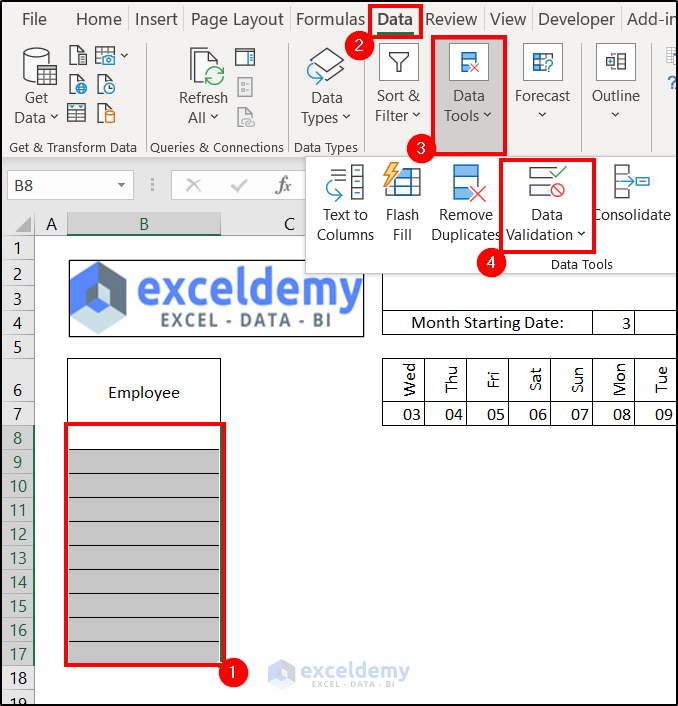
- Select the range for the number of employees you want to insert the roster for. You can always insert or delete rows in between to put up with the changing employee count. We have selected the range B8:B17 for 10 employees for the demonstration and selected Data Validation from the Data Tools group of the Data tab from the ribbon.
- In the Data Validation box’s Settings tab, we have selected a List of “Employee_List” as a Source.
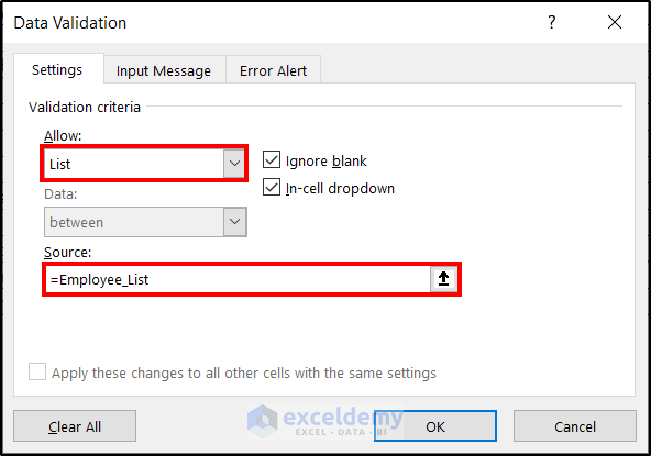
- A drop-down list will be available for each of the selected cells. You can select employee names from here.
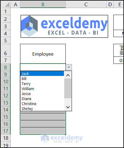
Step 9 – Assemble Starting Shifts
- Merge the cells C6 and C7 for the header.
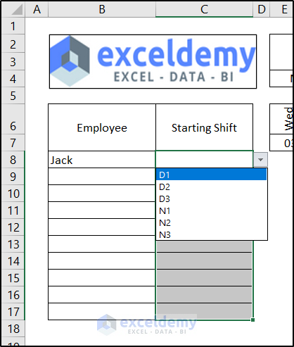
- Select the range C8:C17 and choose Data Validation from the ribbon.
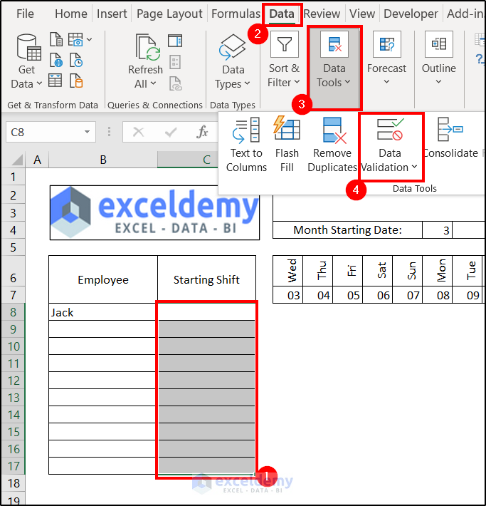
- In the Data Validation box, select List from the Settings tab with the source “Shift_Codes”.
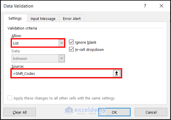
- After clicking on OK, we can select all the shift codes from the available drop-down menu.
Step 10 – Prepare Shifts to Update Based on Starting Shifts
We want the assigned shifts for each day to automatically fill up based on the starting shift. As employees will take turns in the working shifts, we need to rotate through shifts.
- Use the following formula in cell E8:
=IF(OR($C8="",E$7=""),"",IF(D8="",C8,INDEX(Shift_Codes,IF(MATCH(D8,Shift_Codes,0)+1>COUNTA(Shift_Codes),1,MATCH(D8,Shift_Codes,0)+1))))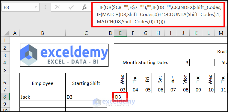
Formula Explanation
IF(OR($C8=””,E$7=””),””,IF(D8=””,C8,INDEX(Shift_Codes,IF(MATCH(D8,Shift_Codes,0)+1>COUNTA(Shift_Codes),1,MATCH(D8,Shift_Codes,0)+1))))
OR($C8=””,E$7=””) checks if either of the cells C8 and E7 has any blank values. Those cells contain IFERROR formulas and may return an empty string depending on the values of other input cells. Also, we have locked columns in the first argument and rows for the second argument. This will be helpful while replicating the whole formula.
The IF(OR($C8=””,E$7=””),””,…) portion of the formula puts an empty string in the cell if both C8 and E7 cells are empty. Otherwise, it moves on to the later portion of the formula.
IF(D8=””,C8,…) comes into play when the previously mentioned logical argument is FALSE. This portion then checks if cell D8 contains a blank value. If it does, then we will just have the value of cell C8. otherwise, it will move on to the next section of the formula. This portion is for the first entries of the roster which will take direct value from the values we will select in column C.
INDEX(Shift_Codes,IF(MATCH(D8,Shift_Codes,0)+1>COUNTA(Shift_Codes),1,MATCH(D8,Shift_Codes,0)+1)) is the value in case the cell D8 isn’t blank (the cell is not in the leftmost column in the roster). Shift_Codes is the array the INDEX function is looking for.
IF(MATCH(D8,Shift_Codes,0)+1>COUNTA(Shift_Codes),1,MATCH(D8,Shift_Codes,0)+1) portion indicates the row number of the INDEX function. If the exact match of cell D8 in the array Shift_Codes is greater than the count of Shift_Codes (counted by the COUNTA function) by at least greater than 2 (compensated by +1), the row number becomes 1 with this IF function.
Otherwise, the row number is MATCH(D8,Shift_Codes,0)+1 which is one higher than the relative position of the value of cell D8 in the Shift_Codes array.
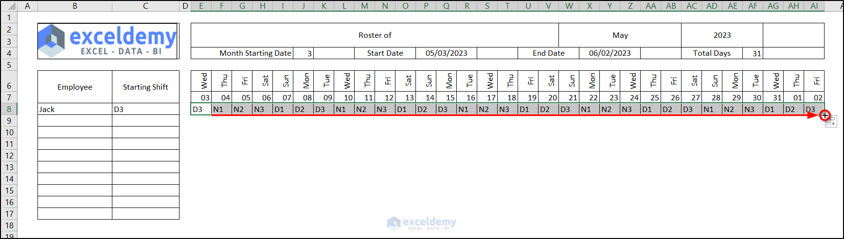
- Replicate the formula by dragging the fill handle icon to cell AI8.
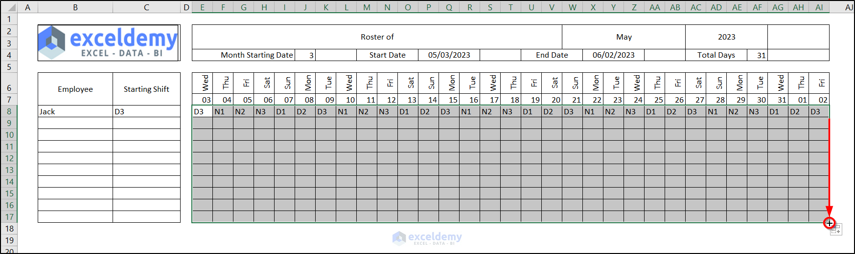
- To fill up the rest of the cells, drag the selection from AI8 to AI17
Step 11 – Create Report Based on Days
- Use the following formula in cell E19:
=COUNTIF(E$8:E$17,"D*")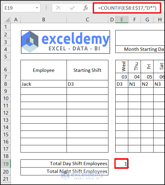
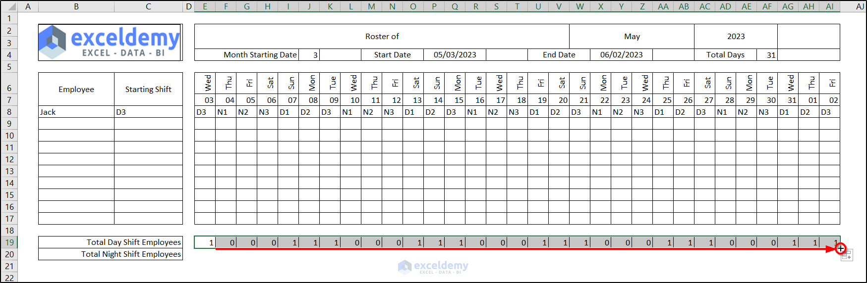
- Replicated the formula in the row until AI19.
- Insert the following formula in cell E20 and drag it to AI20.
=COUNTIF(E$8:E$17,"N*")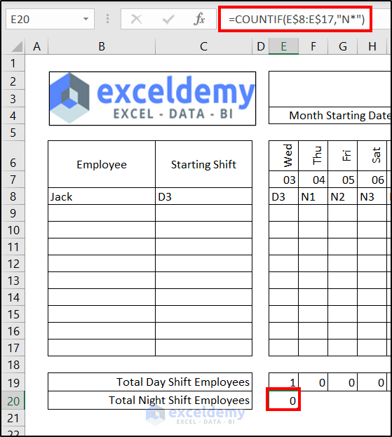
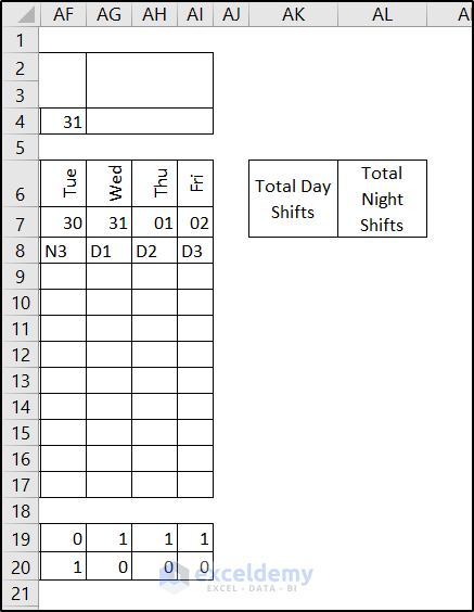
Step 12 – Create Report Based on Employees
- Merge AK6, AK7, and AL6, AL7 for the column headers.
- Copy the following formula in cell AK8:
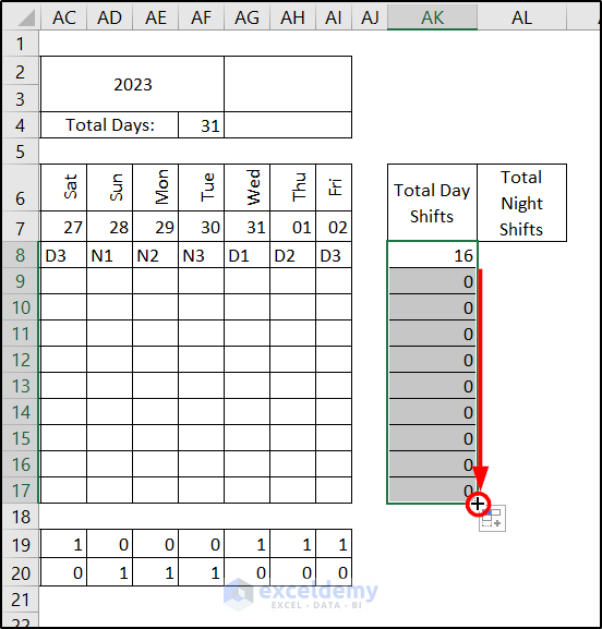
=COUNTIF($E8:$AI8,"D*")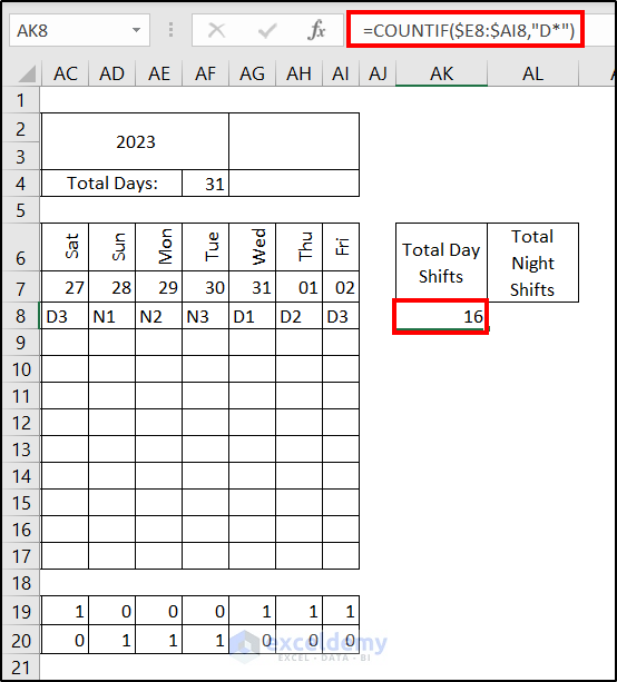
- Drag it down to cell AK17.
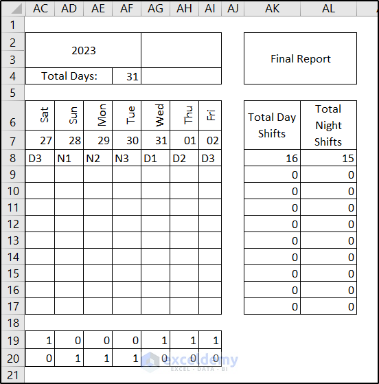
- Similarly, insert the following formula in cell AL8 and drag the fill handle to AL17:
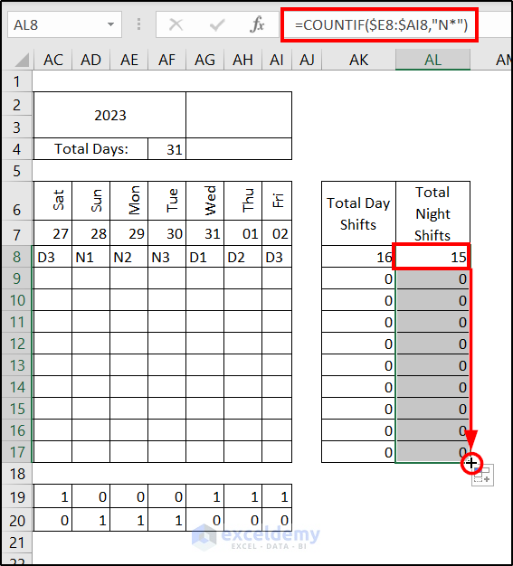
- We have also merged AK2:AL4 to create another header.
Step 13 – Add Formatting to Roster for Shift Types
- Select the range E8:AI17.
- From the Home tab, select Conditional Formatting from the Styles group and New Rule from the drop-down.
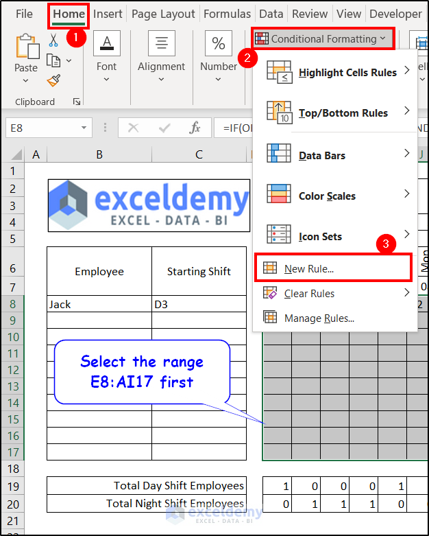
- In the New Formatting Rule box, choose Use a formula to determine which cells to format under Select a Rule Type and insert the following formula in the field:
=LEFT(E8)="N"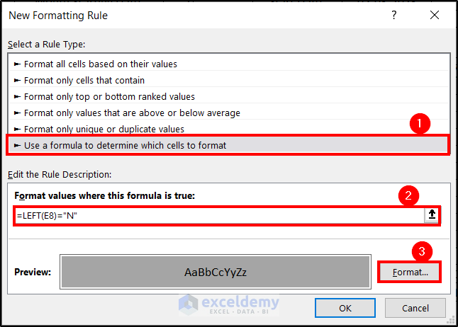
- You can select your format style by clicking on the Format. We opted for a grey fill for the night shifts. After clicking on OK, the night shifts will be colored.
- We have used the same procedure for the day shifts but have inserted the following formula and a light green fill:
=LEFT(E8)="D"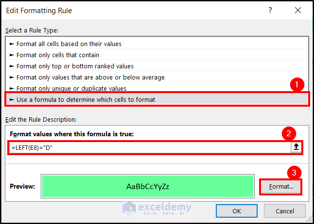
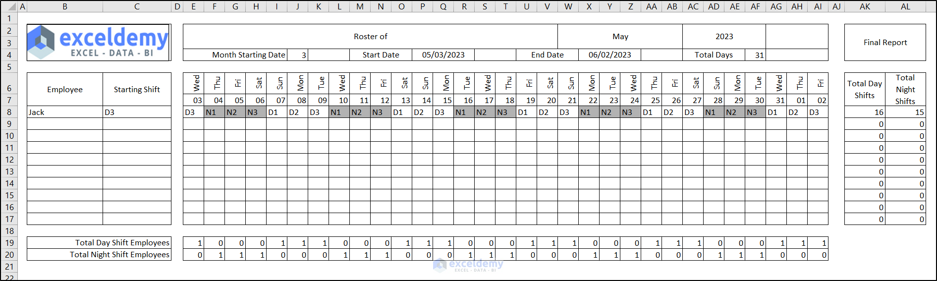
- After clicking on OK, we also have the formats applied for day shifts.
- Format other cells to make the design more presentable.
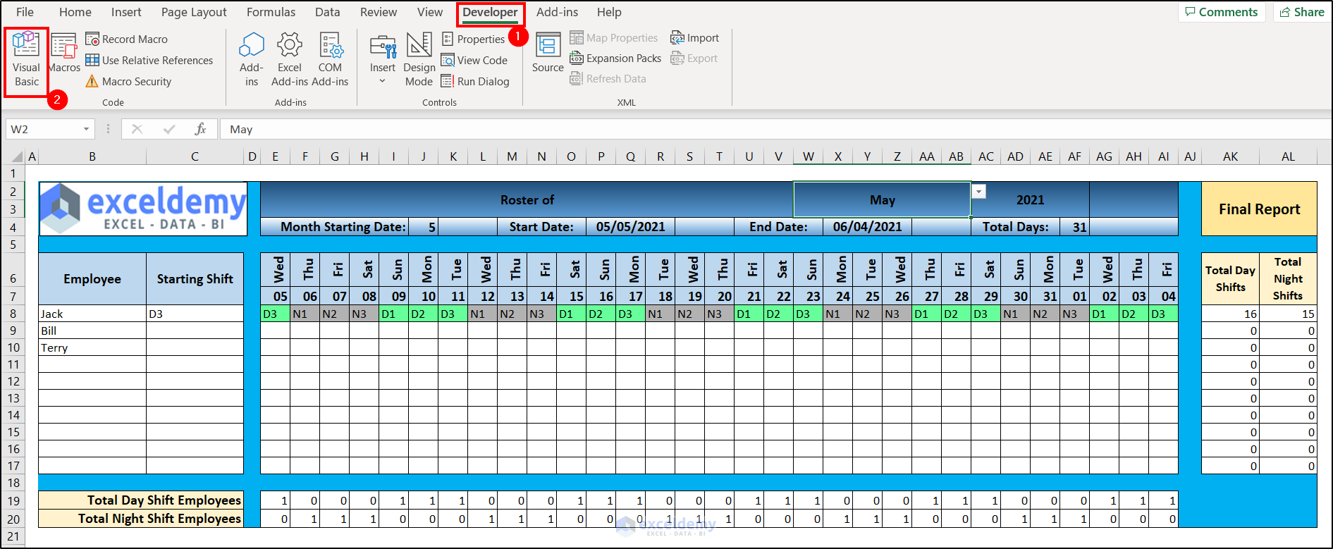
Step 14 – Apply VBA to Automate Sheets for Rest of Months
- To insert a VBA code in a workbook, you select Visual Basic from the Code group of the Developer tab on the ribbon. (You may need to enable this tab in your Settings).
- From the Insert tab of the VBA window, select Module from the drop-down menu.
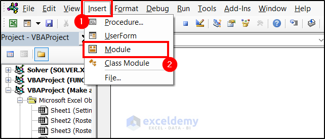
- Copy the following code in the newly created module:
Sub JumpToSheet()
Dim wsht As Worksheet, sht_name As String, wbookX As String, wbookY As Variant
Set wsht = ThisWorkbook.ActiveSheet
sht_name = ActiveSheet.Name
wbookX = Mid(sht_name, 1, Len(sht_name) - 5)
wbookY = Right(sht_name, 4)
    Sheet_Count = ThisWorkbook.Worksheets.Count
    For i = 1 To Sheet_Count
    Sheet_Check = wsht.Range("W2").Value & " " & wsht.Range("AC2").Value
    If Sheets(i).Name = Sheet_Check Then
    Sheets(Sheet_Check).Activate
    End If
    Next i
    If sht_name = "Roster" Then
    wsht.Range("W2").Value = "January"
    wsht.Range("AC2").Value = 2021
    Exit Sub
    Else
    wsht.Range("W2").Value = wbookX
    wsht.Range("AC2").Value = wbookY
    End If
End Sub
Sub CopyToSheet()
Dim wsht As Worksheet, sht_name As String, wbookX As String, wbookY As Variant
Set wsht = ThisWorkbook.ActiveSheet
sht_name = ActiveSheet.Name
wbookX = Mid(sht_name, 1, Len(sht_name) - 5)
wbookY = Right(sht_name, 4)
    Sheet_Count = ThisWorkbook.Worksheets.Count
    ActiveSheet.Copy After:=Worksheets(Sheets.Count)
    If wsht.Range("W2").Value <> "" Then
    ActiveSheet.Name = wsht.Range("W2").Value & " " & wsht.Range("AC2").Value
    End If
    For i = 5 To 35
    If ActiveSheet.Cells(7, i).Value = "" Then
    ActiveSheet.Cells(7, i).EntireColumn.Hidden = True
    Else
    ActiveSheet.Cells(7, i).EntireColumn.Hidden = False
    End If
    Next i
    If sht_name = "Roster" Then
    wsht.Range("W2").Value = "January"
    wsht.Range("AC2").Value = 2021
    Exit Sub
    Else
    wsht.Range("W2").Value = wbookX
    wsht.Range("AC2").Value = wbookY
    End If
End Sub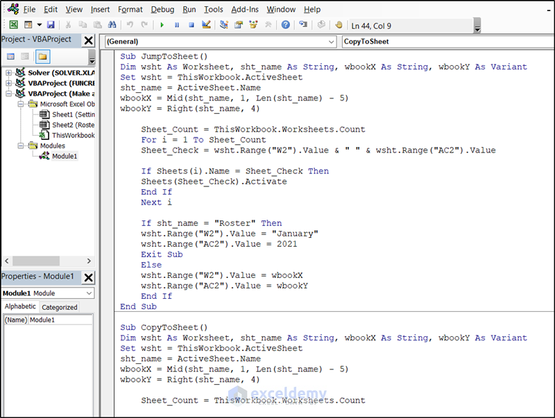
- In the “Roster” sheet, insert the following code:
Private Sub Worksheet_Change(ByVal Target As Range)
Dim wsht As Worksheet
Set wsht = ThisWorkbook.ActiveSheet
Sheet_Count = ThisWorkbook.Worksheets.Count
Check_Sheet = wsht.Range("W2").Value & " " & wsht.Range("AC2").Value
If Not Intersect(Target, Range("W2:AC2")) Is Nothing Then
If Check_Sheet = ActiveSheet.Name Then Exit Sub
    For i = 1 To Sheet_Count
    If Sheets(i).Name = Check_Sheet Then
    Call JumpToSheet
    Exit Sub
    End If
    Next i
    Call CopyToSheet
End If
End Sub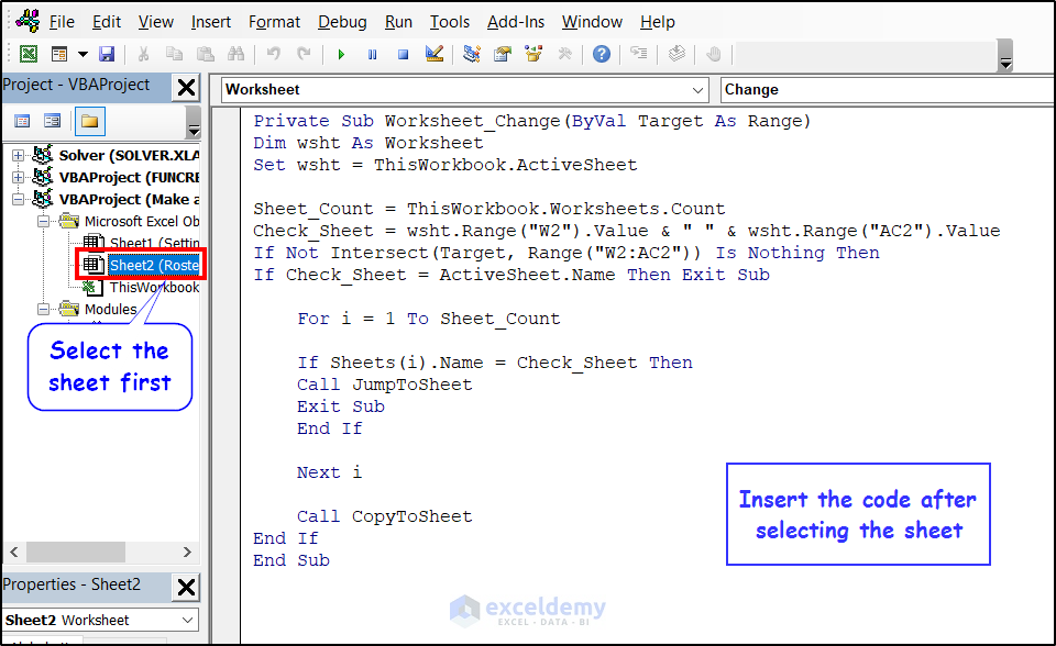
- Once you are done, close the window. Now we can select a new month in cell W2 and a new spreadsheet will open for that with all the formatting and formulas already applied to the cells.
Frequently Asked Questions (FAQs)
- How can I add or remove columns and rows in a roster?
Right-click on the column or row names on the top or left (marked as A, B, 1, 2, etc.) and select Insert from the context menu.
- How can I sort or filter data in a roster to easily view specific information?
Use the Sort & Filter feature available in the Home tab. For more details, check out How to Sort and Filter Data in Excel.
- Is there a way to customize the appearance of the roster, such as changing fonts or adding colors?
Yes, you can customize or format the appearance of cells in a roster just like you would in any other cells in Excel.
- How can I print or share the Excel roster with others?
There is a Print option available in the backstage view which you get after clicking on the File tab on the ribbon. You can also press Ctrl + P. You can either print it or save it as a different file format and share it with others depending on the options you choose.
Things to Remember
- Make sure to keep the changeable named ranges to dynamic ones. It will ensure any new entries will include in the drop-down menus in the roster.
- Consider protecting your spreadsheet in order to prevent any accidental changes in the cells once it is complete.
- You can use the conditional formatting feature for the purpose of error handling too. This is particularly helpful if you ignore data validations and insert values manually.
- While using the formulas, use references and absolute references correctly.
Download Practice Workbook
You can download the workbook used for the demonstration from the link below which you can also use as a template to use.
Get FREE Advanced Excel Exercises with Solutions!

It is great for me. Thank you exceldemy.com.
Dear Khin Soe,
You are most welcome.
Regards
ExcelDemy
Hi Junaed-Ar-Rahman,
I have 4 staff , with 3 working shifts 24/7 5 days in 2 days off. The fourth person only works day shift. I am struggling to find the right setup whereby i need to ensure that if one person is 2 days off that the other 2 will cover the afternoon and night shift. The day shift will be covered by the Team Leader.
Please help.
Hello KRISH
Thanks for reaching out and posting your question. The mentioned schedule can be maintained in several combinations. However, I am presenting a suitable one that will fulfil your requirements.
SHIFT:
Day Shift (D): 8 AM to 4 PM
Afternoon Shift (A): 4 PM to 12 AM
Night Shift (B): 12 AM to 8 AM
MEMBERS:
Staff Rotation Schedule (7-Day Cycle):
Day 1 (Staff D’s day off):
Day 2 (Staff B’s day off):
Day 3 (Staff C’s day off):
Day 4 (Staff A’s day off):
Day 5 (Staff A’s day off):
Day 6 (Staff B’s day off):
Day 7 (Staff C’s day off):
Hopefully, the idea will help you. Good luck!
Regards
Lutfor Rahman Shimanto
Great Tutorial Brother, I need to work out exact amount of hours worked for each employee for the month, we have 4, 2 dayshift guards and 2 nightshift guards. if you can help it would be appreciated
Hello Abdul
Thanks for visiting our blog and sharing your requirements. You wanted to calculate the number of hours worked by each employee in a month. You also mentioned that you have 4 guards, 2 on day and 2 on night shifts. If each shift is 6 hours long and there are 4 shifts in a day, you can calculate the total hours worked by multiplying 6 by the total shits.
You have demonstrated your situation within an Excel file. You can download it by clicking the following link.
DOWNLOAD SOLUTION WORKBOOK
Note: If you want to display more detailed information like calculating exact amount of work time, you must create columns for start and end times. Then, calculate the hours worked for each shift by subtracting the start time from the end time.
I hope these ideas will help you overcome your problem; good luck.
Regards
Lutfor Rahman Shimanto
ExcelDemy
Thank you so Much for your help and time brother
Hello Abdul,
It’s glad to hear and you are most welcome.
Regards
ExcelDemy
Ive used this as a template for my roster. the problem i have now is when i change my month it wont create the new sheet properly. im guessing the visual basic codes wont work if my roster is fairly different? i can change the W2 and AC2 to what my month and year cells are. but the sheets output isnt a replica of my roster sheet
Hello Matthew Richard Raison,
The problem with the VBA code not working for a different roster template could be due to differences in the sheet structure. While using different sheet structure update the VBA code according to you new sheet:
1. Ensure the cells for month and year are correctly referenced (W2 and AC2).
2. Adjust the CopyToSheet subroutine to match the layout and structure of your specific roster sheet.
3. Verify that the new sheet created is an exact replica by manually inspecting the VBA code to ensure all ranges and cell references align with your roster’s layout.
Make these adjustments, and the code should work as intended.
Regards
ExcelDemy
fine
Hello Raj,
Thanks for your appreciation. Keep exploring Excel with ExcelDemy!
Regards
ExcelDemy