In Microsoft Excel, the ISLOGICAL function is generally used to check whether a given argument contains a boolean value (TRUE or FALSE) or not. In this article, you’ll get to learn how you can use this ISLOGICAL function efficiently in Excel with appropriate illustrations.

The above screenshot is an overview of the article, representing a few applications of the ISLOGICAL function in Excel. You’ll learn more about the methods along with the other functions to use the ISLOGICAL function with ease in the following sections of this article.
Introduction to the ISLOGICAL Function
- Function Objective:
The ISLOGICAL function is used to check if a cell contains any boolean or logical values (TRUE or FALSE) or not.
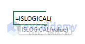
- Syntax:
=ISLOGICAL(value)
- Argument Explanation:
| Argument | Required/Optional | Explanation |
|---|---|---|
| value | Required | Any value or a cell reference or a range of cells. |
- Return Parameter:
A boolean value: TRUE if the function finds a logical value (TRUE or FALSE) in its argument or cell reference, otherwise returns FALSE.
ISLOGICAL Function in Excel: 4 Suitable Examples
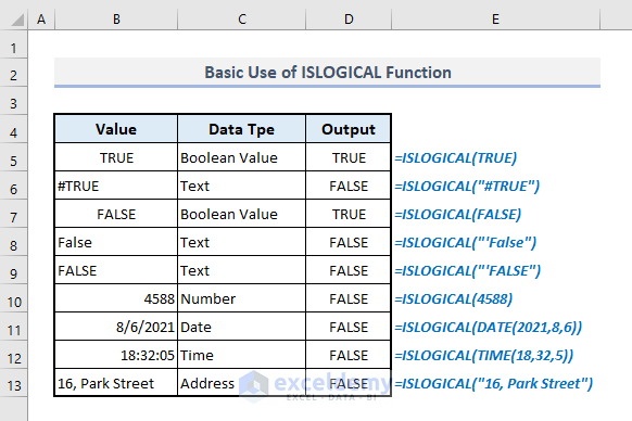
1. Basic Use of ISLOGICAL Function in Excel
In the picture below, a number of data is lying in Column B. We’ll find out which values are logical or boolean ones by applying the ISLOGICAL function in Column D.
For example, the first output in Cell D5 comes with the following formula:
=ISLOGICAL(TRUE)And the function returns TRUE which means TRUE in Cell B5 is a logical function. If it was not a logical function then the function would return FALSE as shown for the second value in Cell B6.
Please don’t forget to use Double-Quotes(“ “) while inputting text data as the argument. For a boolean or a numeric value, you don’t need to use Double-Quotes.
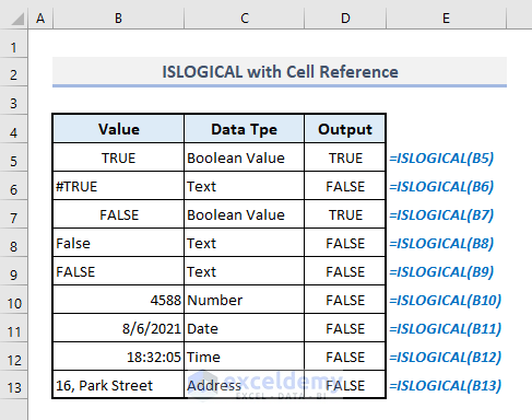
2. Use of ISLOGICAL Function with Cell Reference in Excel
ISLOGICAL function accepts a cell reference too. We’ll now determine the outputs for all the data shown in the previous section by referring to their cell references.
In the output Cell D5, the required formula will be:
=ISLOGICAL(B5)After pressing Enter and auto-filling the rest of the cells in Column D with Fill Handle, you’ll get a similar output as found in the previous example.
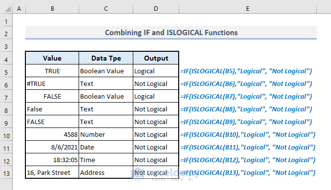
3. Combining IF and ISLOGICAL Functions in Excel
We can incorporate IF and ISLOGICAL functions together to display defined messages. For the values in Column B, the combined formula will return ‘Logical’ for a boolean value and ‘Not Logical’ for a non-boolean value.
For example, the output in Cell D5 will be:
=IF(ISLOGICAL(B5),"Logical", "Not Logical")And the formula will return ‘Logical’ as TRUE is a proper logical or boolean value. Similarly, you can extract the resultant values for all other inputs with their relative cell references.
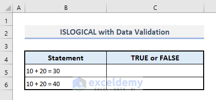
4. ISLOGICAL Function with Data Validation in Excel
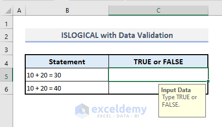
In this section, we’ll see how data validation works with the ISLOGICAL function. In the screenshot below, we have to input TRUE or FALSE based on the statements in Column B. If you type any other text or value then an error message will be displayed.
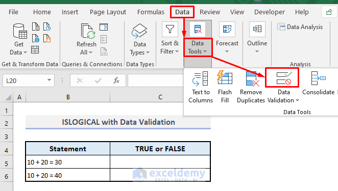
📌 Step 1:
➤ Under the Data ribbon, select the Data Validation command from the Data Tools drop-down.
A dialogue box named ‘Data Validation’ will open up.
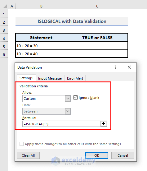
📌 Step 2:
➤ Select the Custom option from the Allow list for Validation Criteria.
➤ In the formula box, type:
=ISLOGICAL(C5)➤ Go to the Input Message tab.
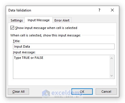
📌 Step 3:
➤ Type “Input Data” for Title.
➤ For the Input message, insert the following text or similar instruction you prefer:
“Type TRUE or FALSE”
➤ Open Error Alert tab.
📌 Step 4:
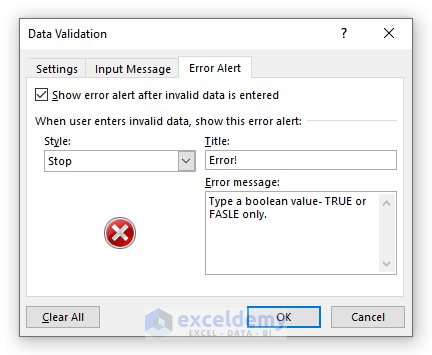
➤ In the title box, type ‘Error!’
➤ Insert the following text as the Error message:
“Type a boolean value- TRUE or FALSE only.”
➤ Press OK.
Now tap on your output cell and you’ll be shown an input message.
📌 Step 5:
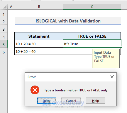
➤ Type a text, such as “It’s True” in Cell C5 for the statement present in Cell B5. An error message will be displayed with the defined texts.
➤ Press Cancel and the message box will disappear.
📌 Step 6:
➤ Now input TRUE only in the output Cell C5 and this time no error message will come up.

💡 Things to Keep in Mind
🔺 ISLOGICAL function is a member of IS group of functions. They are critical in the development of dashboard interfaces and are heavily used with the IF function.
🔺 To input text data you have to use Double-Quotes(“ “) around the argument of the ISLOGICAL function.
🔺 ISLOGICAL function doesn’t return any error no matter what you input as the argument. If it doesn’t recognize a boolean value, it’ll always return FALSE.
Download Practice Workbook
You can download the Excel workbook that we’ve used to prepare this article.
Concluding Words
I hope all of the suitable methods mentioned above to use the ISLOGICAL function will now inspire you to apply them in your Excel spreadsheets with more productivity. If you have any questions or feedback, please let me know in the comment section. Or you can check out our other articles related to Excel functions on this website.
<< Go Back to Excel Functions | Learn Excel
Get FREE Advanced Excel Exercises with Solutions!
