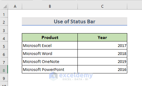
Method 1 – Selecting the Range of Cells to Count Rows with a Value
We have a dataset of Microsoft products and their year versions. We can count the rows containing product names.
STEPS:
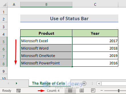
- Select all the rows.
- At the status bar on the bottom right-hand side, an option Count is showing the number of active rows that contain values.
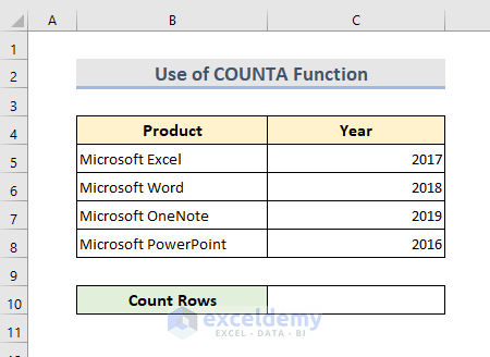
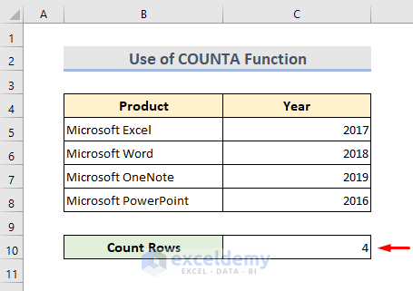
Method 2 – Applying the COUNTA Function to Count Rows with a Value
We are going to count the total number of rows at cell C10 that contain product names.
STEPS:
- Select cell C10.
- Insert the formula:
=COUNTA(B5:B8)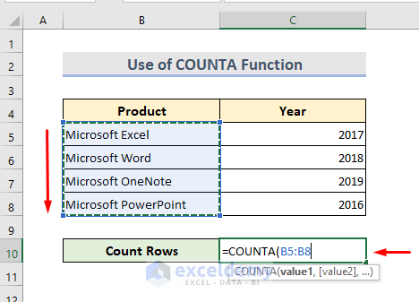
- Hit Enter to see the result.
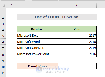
Method 3 – Counting Rows with Numerical Values with the COUNT Function in Excel
We have a dataset of Microsoft products with their year version. We are going to count the numerical values at cell C10.
STEPS:
- Select cell C10.
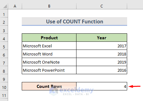
- Insert the formula:
=COUNT(B5:C8)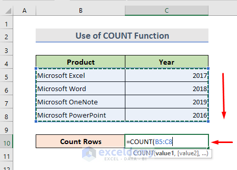
- Press Enter.
Method 4 – Applying the COUNTIF Function to Count Rows with a Text Value in Excel
With the help of a wild character Asterisk (*), we can apply the COUNTIF function to count rows with text values.
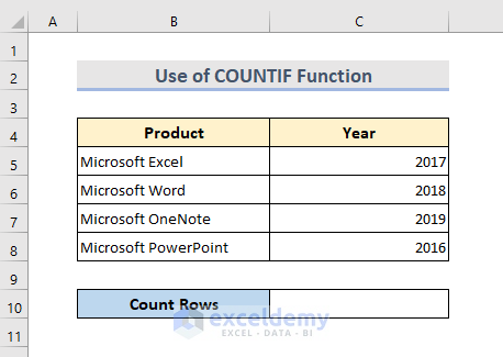
STEPS:
- Select cell C10.
- Use the formula:
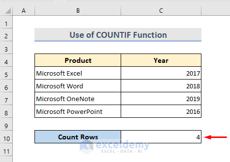
=COUNTIF(B5:B8,"*")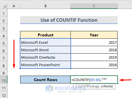
- Hit Enter for the result.
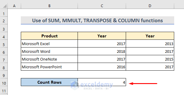
Method 5 – Using Excel SUM, MMULT, TRANSPOSE, and COLUMN Functions to Count Rows with a Specific Value
We have a worksheet containing Microsoft products and their year version. We will find out the number of rows that contain “2017” in cell C10.
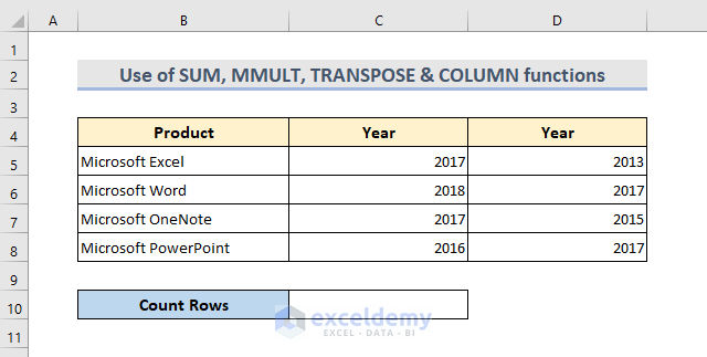
STEPS:
- Select cell C10.
- Use the formula:
=SUM(--(MMULT(--(C5:D8=2017),TRANSPOSE(COLUMN(C5:D8)))>0))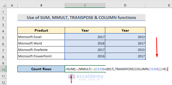
- Hit Enter to see the result.
➤➤➤ Simplification of the Formula:
- The logical criterion of the formula is:
=--(C5:D8=2017)This generates the TRUE/FALSE array result and the double negative (—) compels the values of TRUE/FALSE in 1 & 0 respectively.
- The array of 4 rows and 2 columns (4*2 array) goes to the MMULT function as Array1.
- To get the column number in an array format, we use the COLUMN function.
=COLUMN(C5:D8)- To transform the column array format into a row array, we use the TRANSPOSE function.
=TRANSPOSE(COLUMN(C5:D8))- The SUM function counts the rows with values.
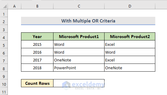
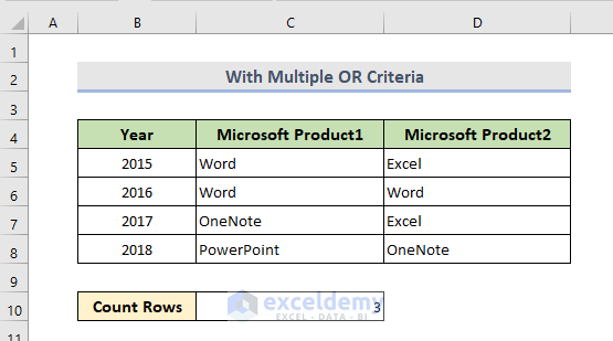
Method 6 – Counting Rows with Multiple OR Criteria in Excel
We have to count the rows where Product1 is Word or Product2 is Excel.
STEPS:
- Select cell C10.
- Insert the formula:
=SUMPRODUCT(--((C5:C8="Word")+(D5:D8="Excel")>0))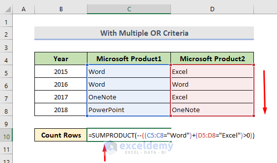
➤ NOTE: Here the two logical criteria are attached by the sign plus (+) as addition is required in Boolean algebra. The first logical criteria test if the product1 is Word and the second criteria test if the product2 is Excel. We won’t use the SUMPRODUCT function only as it double counts rows with both Word & Excel. We use double negative(—) as it compels the values of TRUE/FALSE in 1 & 0 respectively with “>0”. A single array of 1s & 0s is created inside the SUMPRODUCT function.
- Hit Enter for the result.
.
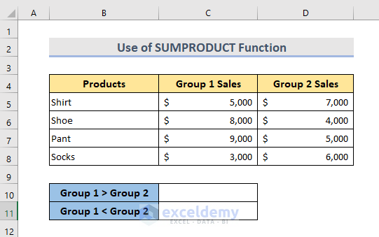
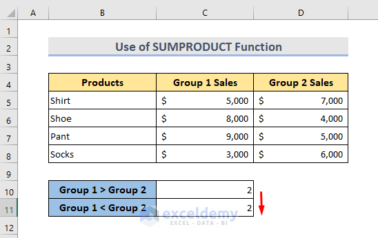
Method 7 – Using the SUMPRODUCT Function to Count Rows that Meet Internal Criteria
We have a dataset of products and the sales record of Group 1 and Group 2.
Criteria:
- Group 1 > Group 2
- Group 2 > Group 1
STEPS:
- Select cell C10.
- For the Group 1 > Group 2 condition, use the formula:
=SUMPRODUCT(--(C5:C8>D5:D8))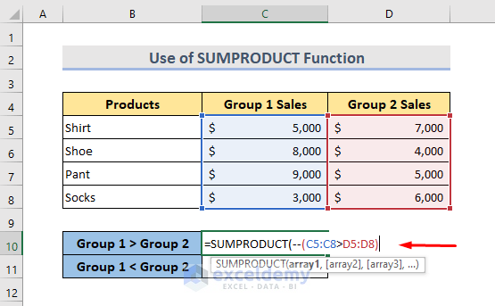
- Hit Enter.
- For the Group 2 > Group 1 condition, use the formula:
=SUMPRODUCT(--(C5:C8<D5:D8))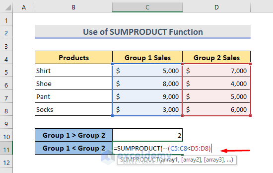
- Hit Enter and see the result.
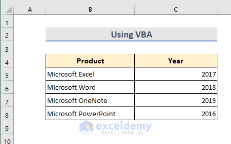
Method 8 – Using VBA to Count Rows with Value in Excel
We are going to count all the used rows that contain data.
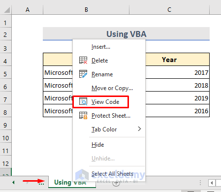
STEPS:
- Go to the sheet tab and right-click on the name of the active sheet.
- Select View Code.
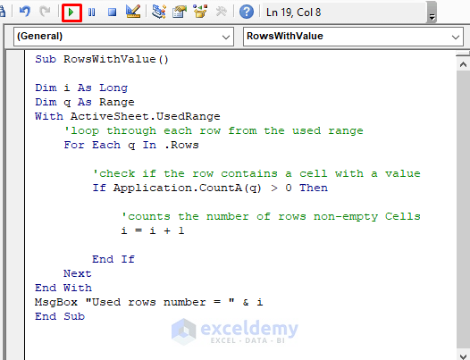
- A VBA Module window pops up.
- Insert the following code in it.
Option Explicit
Sub RowsWithValue()
Dim i As Long
Dim q As Range
With ActiveSheet.UsedRange
'loop through each row from the used range
For Each q In .Rows
'check if the row contains a cell with a value
If Application.CountA(q) > 0 Then
'counts the number of rows non-empty Cells
i = i + 1
End If
Next
End With
MsgBox "Used rows number = " & i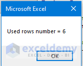
End Sub- Click on the Run option.
- We can see the final counting result in a short message box.
Download the Practice Workbook
<< Go Back to Count Rows | Formula List | Learn Excel
Get FREE Advanced Excel Exercises with Solutions!
