Excel is the most widely used tool for dealing with massive datasets. We can perform myriads of tasks of multiple dimensions in Excel. Dave Ramsey, a prominent finance personality from the USA suggested repaying multiple loans following the snowball method. In this article, I will show you how to create a Dave Ramsey debt snowball spreadsheet in Excel.
Introduction to the Snowball Method
The Snowball method is a loan repayment method where you pay a minimum amount to every loan and use the rest of the amount to repay the lowest loan. Let us see an example of this method. If you have three outstanding debts of $10, $20, and $30, the minimum payment is $2 for each. Then, you will pay the total minimum amount of $6 and may choose to include additional money towards the $10 debt.
This additional amount will be applied to the lowest debt. Whenever we finish paying the lowest debt, then this amount will be applied to the second-lowest debt. Thus, it creates a snowball effect to make the payment faster
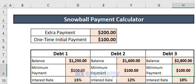
This is the dataset for today’s article. We have 3 debts. I will show the repayment schedule of these debts using the snowball payment calculator in Excel. Please note that the total payment each month is $500. After a minimum payment of $100 for each loan, there will be an extra $(500-3*100) or $200 which will be used for the lowest debt. Additionally, I have a one-time payment of $100 too.
Step 1: Calculating Payment Amount for 1st Month of Lowest Debt to Create a Dave Ramsey Debt Snowball Spreadsheet in Excel
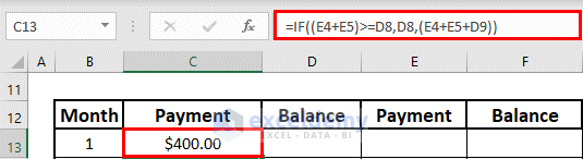
The first step is to calculate the amount that you are going to pay for the 1st month of the lowest debt. To do so,
- Go to C13 and write down the following formula
=IF((E4+E5)>=D8,D8,(E4+E5+D9))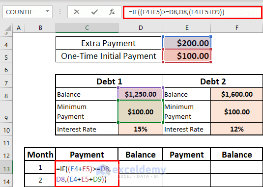
- Then, press ENTER to get the output.
Read More: Debt Snowball Vs Debt Avalanche Method in Excel Spreadsheet
Step 2: Finding Balance After 1st Month of Lowest Debt
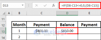
The next step is to find the balance for 1st month of the lowest debt. To calculate it,
- Go to D13 and write down the following formula
=IF(D8-C13<=0,0,(D8-C13))
- Then, press ENTER to get the output.
Step 3: Calculating Payment Amount for 1st Month of 2nd Lowest Debt to Create a Dave Ramsey Debt Snowball Spreadsheet in Excel
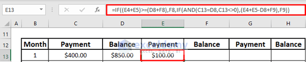
The next step is to calculate the amount that you are going to pay for the 2nd lowest debt. To do so,
- Go to E13 and write down the following formula
=IF((E4+E5)>=(D8+F8),F8,IF(AND(C13=D8,C13<>0),(E4+E5-D8+F9),F9))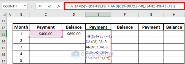
Formula Breakdown:
- AND(C13=D8,C13<>0) → This is the logical test.
- Output: FALSE
- (E4+E5)>=(D8+F8) → This is another logical test.
- Output: FALSE
- IF((E4+E5)>=(D8+F8),F8,IF(AND(C13=D8,C13<>0),(E4+E5-D8+F9),F9))
- Output: 100.
- Then, press ENTER to get the output.
Step 4: Finding Balance After 1st Month of 2nd Lowest Debt
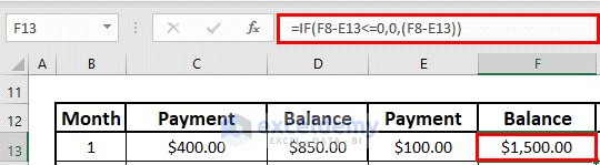
The next step is to find the remaining balance for the 1st month of the 2nd lowest debt. To do so,
- Go to F13 and write down the following formula
=IF(F8-E13<=0,0,(F8-E13))
- Then, press ENTER to get the output
Step 5: Calculating Payment Amount for 1st Month of Last Debt to Create a Dave Ramsey Debt Snowball Spreadsheet in Excel
The next step is to calculate the amount that you are going to pay for the 1st month of the last debt. To do so,
- Go to G13 and write down the following formula
=IF((E4+E5)>=(F8+H8+D8),H8,IF(AND(E13=F8, E13<>0),(E4+E5-F8-D8+H9),H9))
- Then, press ENTER to get the output.

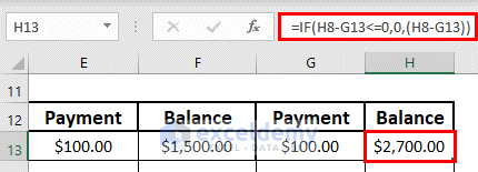
Step 6: Finding Balance After 1st Month of Last Debt
Next, I will show how to find the remaining balance after the 1st month of the last debt. For this,
- Go to H13 and write down the following formula
=IF(H8-G13<=0,0,(H8-G13))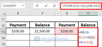
- Then, press ENTER to get the output.
Step 7: Determining Payment Amount for Subsequent Months of Lowest Debt
Now, I will show how to calculate the amounts that you need to pay for the subsequent months. First of all, I will use a formula for the lowest debt.
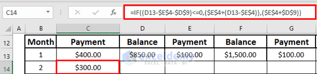
- Go to C14 and write down the following formula
=IF((D13-$E$4-$D$9)<=0,($E$4+(D13-$E$4)),($E$4+$D$9))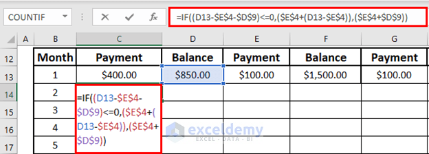
- Then, press ENTER to get the output.
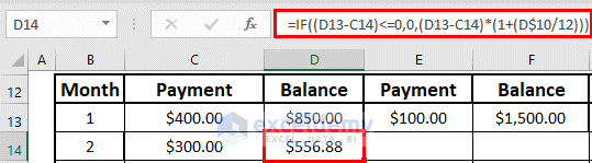
Step 8: Calculating Balance After Subsequent Months of Lowest Debt
Next, I will calculate the remaining balance after subsequent months of the lowest debt. This balance will include the interest applied in the previous months.
- Go to D14 and write down the following formula
=IF((D13-C14)<=0,0,(D13-C14)*(1+(D$10/12)))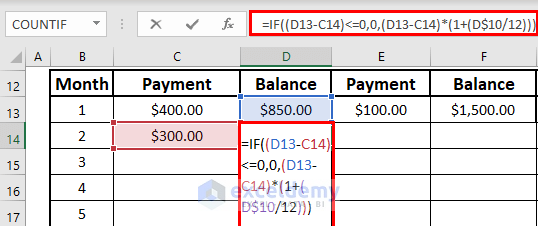
- Then, press ENTER.
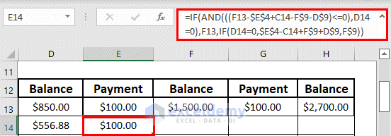
Step 9: Determining Payment Amount for Subsequent Months of 2nd Lowest Debt
Now, you will see how to determine the amount that you need to pay for the subsequent months of the 2nd lowest debt. For this,
- Go to E14 and write down the following formula
=IF(AND(((F13-$E$4+C14-F$9-D$9)<=0),D14=0),F13,IF(D14=0,$E$4-C14+F$9+D$9,F$9))
Formula Breakdown:
- AND(((F13-$E$4+C14-F$9-D$9)<=0),D14=0) → This is the 1st logical test
- Output: FALSE
- IF(D14=0,$E$4-C14+F$9+D$9,F$9)
- Output: 100
- IF(AND(((F13-$E$4+C14-F$9-D$9)<=0),D14=0),F13,IF(D14=0,$E$4-C14+F$9+D$9,F$9))
- Output: 100
- Now, press ENTER to get the output.
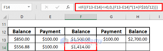
Step 10: Finding Balance After Subsequent Months of 2nd Lowest Debt
The next step is the calculation of the balance after the subsequent months of 2nd lowest debt. These payments include the interests of previous months. To calculate it,
- Go to F14 and write down the following formula
=IF((F13-E14)<=0,0,(F13-E14)*(1+(F$10/12)))
- Then, press ENTER to get the output.
Step 11: Calculating Payment Amount for Subsequent Months of Last Debt
This time, I will calculate the amount that you need to pay for the subsequent months of the last debt. To do so,
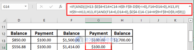
- Go to G14 and write down the following formula
=IF(AND(((H13-$E$4+E14+C14-H$9-F$9-D$9)<=0),F14+D14=0),H13,IF(H$9>=H13,H13,IF(AND(F14=0,D14=0),$E$4-E14-C14+H$9+F$9+D$9,H$9)))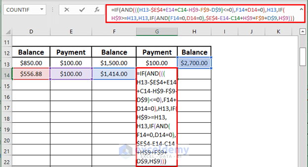
Formula Breakdown:
- AND(((H13-$E$4+E14+C14-H$9-F$9-D$9)<=0),F14+D14=0) → This is the 1st logical test.
- Output: FALSE
- H$9>=H13 → This is the 2nd logical test.
- Output: FALSE
- AND(F14=0,D14=0) → This is the 3rd logical test.
- Output: FALSE
- IF(AND(((H13-$E$4+E14+C14-H$9-F$9-D$9)<=0),F14+D14=0),H13,IF(H$9>=H13,H13,IF(AND(F14=0,D14=0),$E$4-E14-C14+H$9+F$9+D$9,H$9)))
- Output: 100
- Then, press ENTER to get the output.
Step 12: Determining Balance After Subsequent Months of Last Debt
Finally, I will calculate the remaining balance after subsequent months of the last debt. For this,
- Go to H14 and write down the following formula
=IF((H13-G14)<=0,0,(H13-G14)*(1+(H$10/12)))
- Then, press ENTER to get the output.

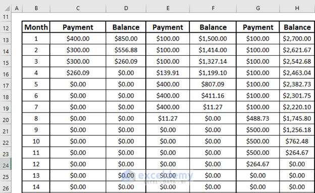
- Finally, use Excel Fill Handle tool to fill automatically. The final result will look like this.
Things to Remember
- Do not forget to repay a minimum amount on all loans
- Use the absolute reference to lock a cell with an Excel formula.
Download Practice Workbook
Download this workbook and practice while going through the article.
Conclusion
In this article, I have explained how to create a Dave Ramsey debt snowball spreadsheet in Excel. I hope it helps everyone. If you have any suggestions, ideas, or feedback, please feel free to comment below. Please visit Exceldemy for more useful articles like this.
Related Articles
- Debt to Income Ratio Calculator in Excel
- Credit Card Debt Reduction Calculator for Excel
- Create Pay off Credit Card Debt Calculator in Excel
- Create Debtors Ageing Report in Excel Format
<< Go Back to Debt Template | Finance Template | Excel Templates
Get FREE Advanced Excel Exercises with Solutions!

How do I add additional Debt columns past Debt 3? I tried to copy/drag the cells to create a new Debt (4), but I get an error in the Payment column for Debt 4. It doesn’t add the Minimum Payment from Debt 4 to the Payment due. Same error occurs with additional Debts added.
Hello Scott Wolfe,
The template in the article is built for exactly 3 debts, so dragging the formulas to create “Debt 4” won’t work automatically. The Payment formulas reference fixed cells (D9, F9, H9 for minimum payments and D8, F8, H8 for balances), so when you add a new debt, Excel doesn’t include your new cells.
To make Debt 4 work, you must manually update the references.
For example, if your new Debt 4 minimum payment is in J9, update the total minimum-payment formula from:
=D9+F9+H9 to: =D9+F9+H9+J9
(or =SUM(D9:J9))
Then adjust the last-debt Payment formula (originally in G13):
Original (Debt 3):
=IF((E4+E5)>=(F8+H8),H8,IF(AND(C13=F8,C130),(E4+E5-F8+H9),H9))
New for Debt 4: change all references from H8/H9 → J8/J9 and from the previous payment cell (C13 or G13) → the Debt 3 payment cell.
Regards,
ExcelDemy