Create a Timeline in Excel with Milestones (With Easy Steps)

This article illustrates how to create a timeline in Excel with milestones in 8 quick steps. It is always a good idea to make a timeline with certain milestones for your projects. This will help you to keep track of your progress easily. It may also motivate you to work more efficiently to meet the milestones. Have a quick look through this article so that you too can create a timeline with milestones in Excel pretty easily.

How to Create a Timeline with Milestones in Excel

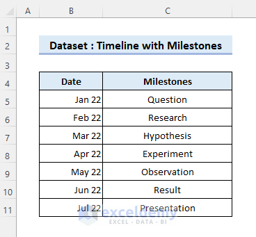
Consider the following dataset. It contains the 7 fundamental steps of a scientific study. Now, assume you want to create a timeline in Excel using the steps as the milestones for a particular problem.

You can easily do that using the Excel Line Chart with Markers. Follow the steps below to quickly learn how to do that.

Create a Timeline in Excel with Milestones Using Line Chart with Markers: 8 Easy Steps

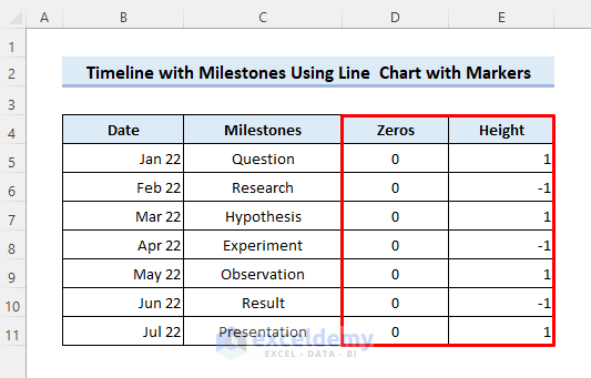
Step-1: Create Two Helper Columns

First, you need to create two helper columns. Create a new column for zeros adjacent to the Milestones column. Next, enter 0 in each cell of that column.
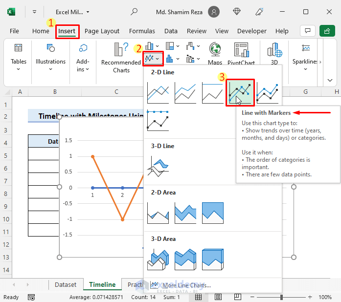
Then, create a Height column adjacent to the Zeros column. After that, enter 1 and -1 repeatedly in the cells of that column. You can discard the negative signs to keep all of the milestones on the same side in the chart.

Step-2: Insert a Line Chart with Markers

Now, select the zeros and ones (D5:E11) from the helper columns. Next, select Insert >> 2-D Line >> Line with Markers as shown below. Then a Line Chart will be created.

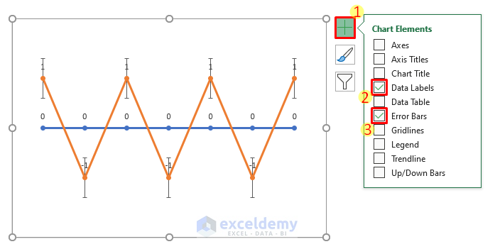
Step-3: Enable/Disable Some Chart Elements

Now, click on the + sign at the upper right corner of the chart. If the sign is not visible then click on the chart area. After that, it will be visible again.
Then, uncheck all Chart Elements except the Data Labels and the Error Bars. You should check these two checkboxes if they are not already checked.

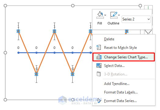
Step-4: Change the Chart Type for a Series

Now, click on the yellow-colored line chart that goes up and down as shown below. Then, make sure that all of the data points are selected. Next, right-click and select Change Series Chart Type.

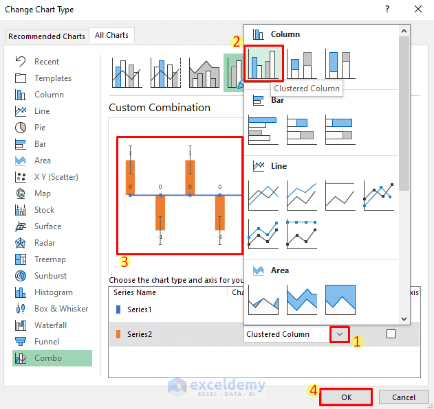
After that, select the Clustered Column chart type from the pop-up list. You will see a preview of what the new chart will look like.
Make sure you are doing this for the correct series by noticing the color of it. Next, select OK. After that, it will be converted to a column chart.

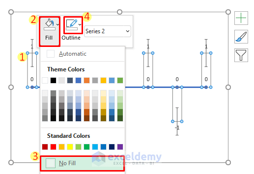
Step-5: Hide the Clustered Column Chart

Next, click on any one of the columns in the chart. Then make sure that all of the columns are selected.
After that, right-click and select the dropdown for Fill Color. Then, select No Fill. Next, click on the Outline dropdown and select No Outline.

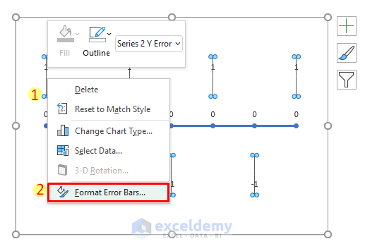
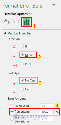
Step-6: Format the Error Bars

Now, click on any one of the Error Bars and ensure that all of them are selected. Then right-click and select Format Error Bars. Then a dialog box will pop up on the right side of your Excel window.

Next, choose the Direction for the Vertical Error Bar as Minus, No Cap for End Style, and set the Error Amount percentage to 100%.

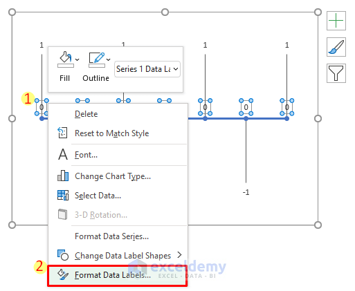
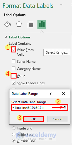
Step-7: Add the Data Labels

After that, click on any one of the data labels for the Zeros column and make sure that all of them are selected. Next, right-click and select Format Data Labels.

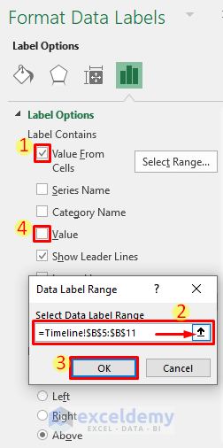
Now, check the Value From Cells Then, an input dialog box will pop up. Next, use the upward arrow to select the Date values (B5:B11) and then click OK. Next, uncheck the Value checkbox.

Now, click on any one of the data labels for the Height column and ensure that all of them are selected. Next, right-click and select Format Data Labels as in the earlier step.

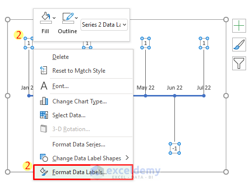
Next, select the Milestones in the same way as earlier and press OK.

Step-8: Make the Timeline Presentable

Finally, you can make the timeline a bit more presentable. Drag the data labels to fit them properly or change the label colors. After that, you will have your presentable timeline with milestones as shown in the picture below.

Download Practice Workbook

You can download the practice workbook from the download button below.

Creating Timeline with Milestones.xlsx

Things to Remember

Always make sure that all of the data points or the data labels are selected to change them altogether.
Follow the steps as numbered to avoid any undesired results along the way.

Conclusion

Now you know how to create a timeline with milestones in Excel with simple steps. Please let us know if this article has helped you to get the desired results. You can also use the comment section below for further queries or suggestions.

<< Go Back to Timeline in Excel | Learn Excel

Get FREE Advanced Excel Exercises with Solutions!