How to Create Animated Charts in Excel (with Easy Steps)

Get FREE Advanced Excel Exercises with Solutions!

Excel is used in every commercial organization to create databases and organize data as needed. Thankfully, a lot of us utilize Excel in our professional settings. Additionally, it’s interesting to note that Excel makes it simple to create animations for better display. Animation charts use animated and progressive illustrations of the data to help the viewer better interpretation of the charts. For the animation charts to move and change dynamically, further work and understanding of macros are needed. We can generate animated charts in Excel with the help of VBA Macros. You may think it’s tough to make one animated chart. Believe it or not, it’s going to be fun to create animated charts in Excel. In this article, we’re gonna show you simple steps to make animated charts in Excel. Let’s get started.

Table of Contents hide

Download Practice Workbook

4 Steps to Create Animated Charts in Excel

Step 1: Setting up a Chart with Helper Column

Step 2: Formatting the Chart

Step 3: Employing VBA Code

Step 4: Entering a Button to Generate the Animation

Practice Section

Conclusion

Download Practice Workbook

Download the following practice workbook. It will help you to realize the topic more clearly.

Generating Animated Charts.xlsm

4 Steps to Create Animated Charts in Excel

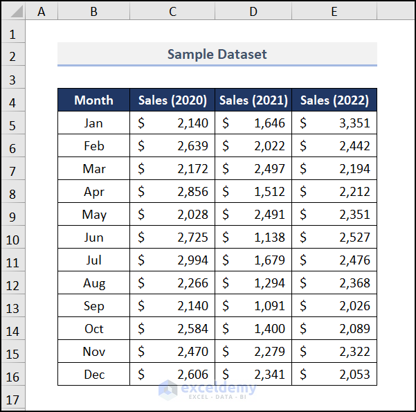
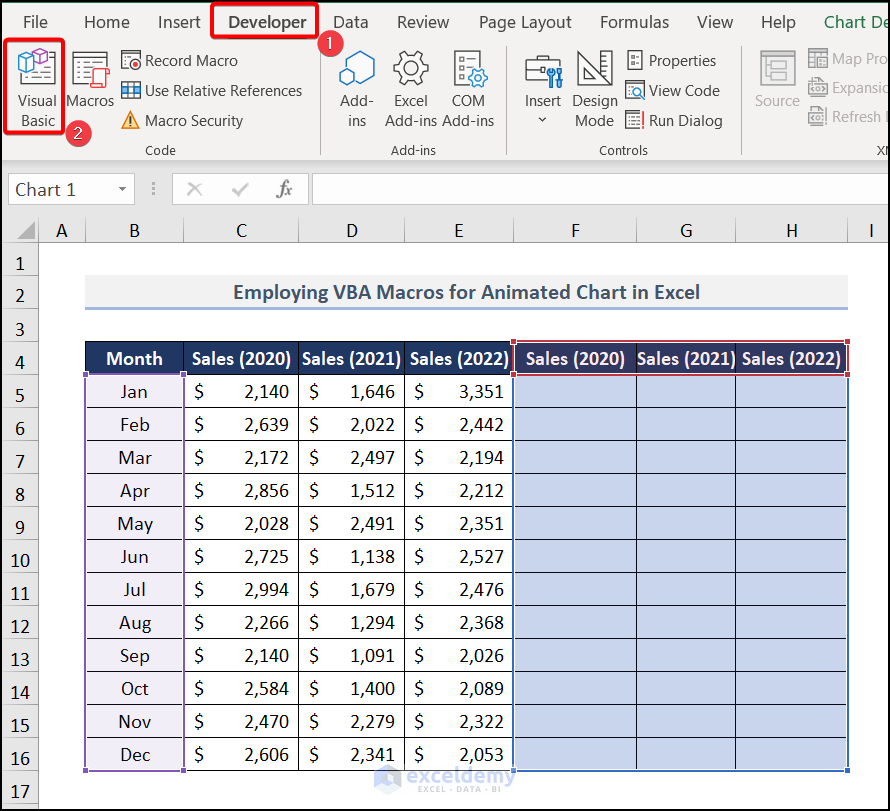
Mainly, an animated chart can be created through VBA code. But before going to the coding section, you need to create a dataset. Here, we have taken a dataset of Month-wise Sales for 3 consecutive years 2020, 2021, and 2022. We will generate a chart that changes with the timing strap. That means we are going to make an animated chart.

Not to mention, we have used the Microsoft 365 version. You may use any other versions at your convenience.

Step 1: Setting up a Chart with Helper Column

At the very beginning, we need to insert the three “Sales” columns with what we create in the chart.

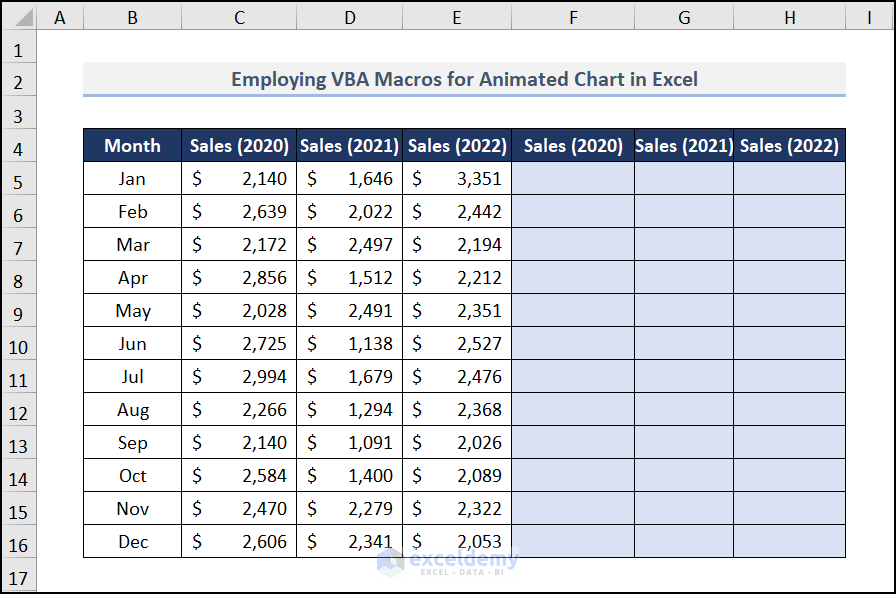
Note: You can highlight the helper columns for better visualization.

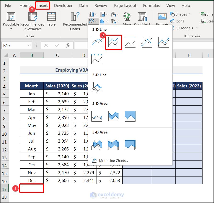
Initially after, move to a blank cell. Then, navigate to the Insert tab >> under the Charts section choose Insert Line or Area Chart >> pick up Stacked Line.

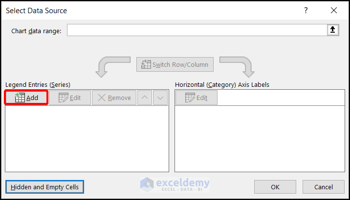
Apparently, a chart has been created. Right-click on the chart and click on Select Data.

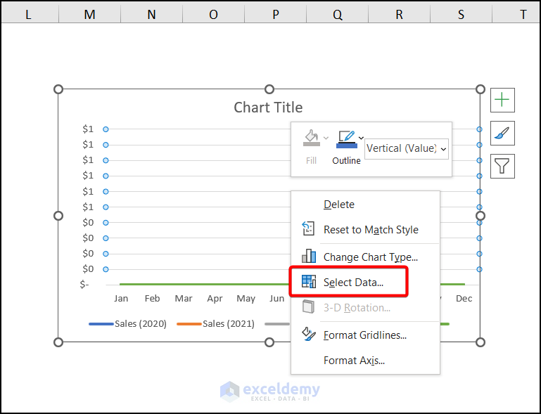
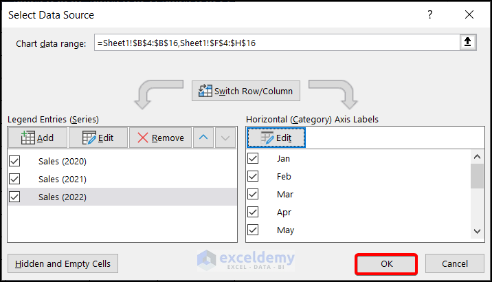
Consequently, the Select Data Source dialog box pops out. Choose Add from the Legend Entries (Series).

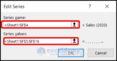
At this moment, you will see the Edit Series window. In the Series Name box, choose the Sales (2020), and in the Series values box, select the data range from $F$5:$F$16. Press OK.

Sequentially, select all the “Sales” columns like the above procedure.

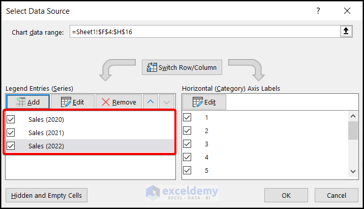
Moreover, in the Horizontal (Category) Axis Labels, move to Edit.

Subsequently, the Axis Labels dialog box pop out. Select the data range from $B$5:$B$16. Click OK.

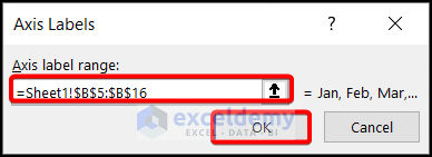
Finally, hit OK in the Select Data Source window.

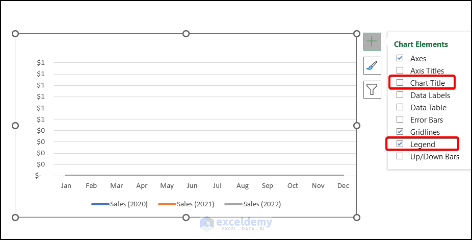
Step 2: Formatting the Chart

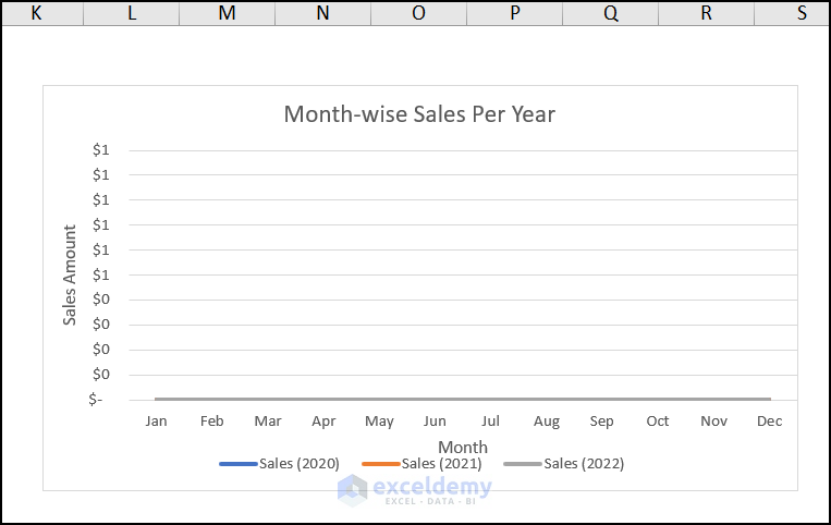
You have to modify your chart appearance by creating the Chart Title, the Axis Titles, and the Legend at the bottom.

Eventually, your chart will look something similar to the image below.

Step 3: Employing VBA Code

At this moment, it’s high time we entered the VBA code for the animated charts.
Firstly, hover over the Developer tab >> choose Visual Basic.

Consequently, choose the Insert tab >> Module>> Module1.

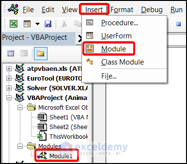
In Module 1, you will see the General box. Write the following VBA code there.

Sub AnimationChart()
    Const SR As Long = 5
    Dim LR As Long
    Dim RN As Long
    LR = Range("C" & SR).End(xlDown).Row
    Range("F" & SR, "H" & LR).ClearContents
    DoEvents
    Application.Wait (Now + TimeValue("00:00:1"))
    For RN = SR To LR
        DoEvents
        Range("F" & RN, "H" & RN).Value = Range("C" & RN, "E" & RN).Value
        Application.Wait (Now + TimeValue("00:00:1"))
        DoEvents
    Next RN
End Sub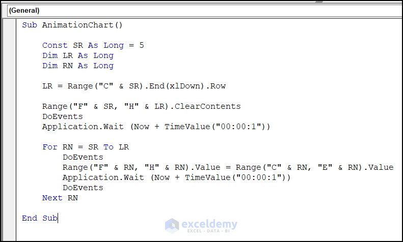

Code Breakdown

We declare the variables first. We set the Constant as SR representing Starting Row. In our case, it is 5. The LR and RN are also variables referring to the values of the Last Row and Row Number respectively.

LR = Range(“C” & SR).End(xlDown).Row→command removes all the values of the associated column (F: H).

Range(“F” & SR, “H” & LR).ClearContents→picked the range of cells, started showing the cell values row by row and filled the blank columns of F to H.

We have set the Time delay to 1 second, which will help us show the data at a 1-second delay, which gives a dynamic vibe to the chart.

Step 4: Entering a Button to Generate the Animation

At this stage, you can add a button utilizing the Form Controls in your worksheet.

After adding the button, right-click on the Animation button and choose Assign Macro from the Context Menu.

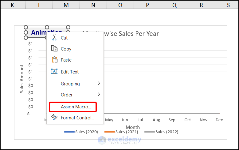
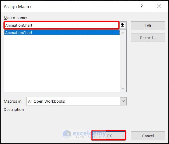
Sequentially, the Assign Macro dialog box appears. Select the Macro name as AnimationChart. Press OK.

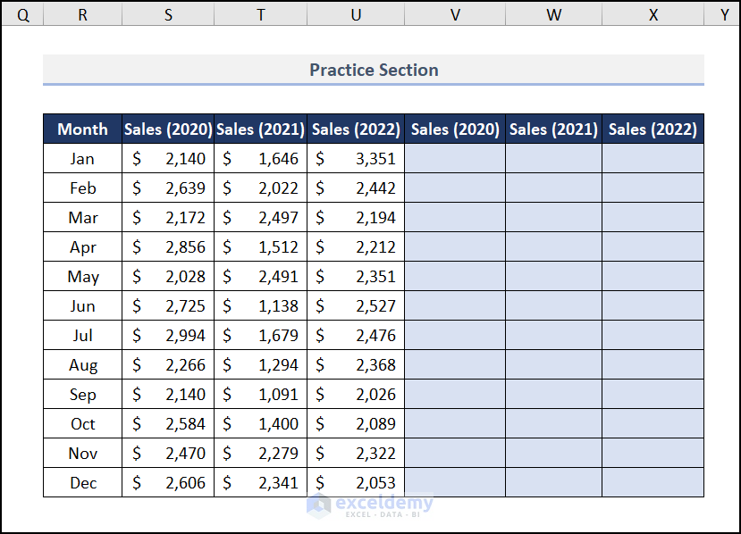
Finally, your animated chart is ready. Click on the Animation button and get the result like the below gif.

Practice Section

We have provided a practice section on each sheet on the right side for your practice. Please do it by yourself.

Conclusion

That’s all about today’s session. And these are some easy steps to create an animated chart in Excel. Please let us know in the comments section if you have any questions or suggestions. For a better understanding please download the practice sheet. Visit our website Exceldemy, a one-stop Excel solution provider, to find out diverse kinds of excel methods. Thanks for your patience in reading this article.