Professional business owners who use Six Sigma to design their operation outline and significantly lower the errors sometimes use a control chart in Excel to help them supervise the process. The control chart comprises elements like Upper Control Limit, lower control limit, mean, etc. The upper control limit is the highest limit for data to keep the process optimum which can be calculated by using the average and standard deviation of data. In this article, we will the stepwise procedures to calculate upper limit control limit with a formula in Excel.
How to Calculate Upper Control Limit with Formula in Excel (With Easy Steps)
In this section, we will discuss the stepwise procedures to calculate the upper control limit with a formula in Excel. The general formula for determining the upper control limit is:
UCL = Average + (3*Standard Deviation)Without any dilemma, let’s jump to the procedures to calculate the upper control limit.
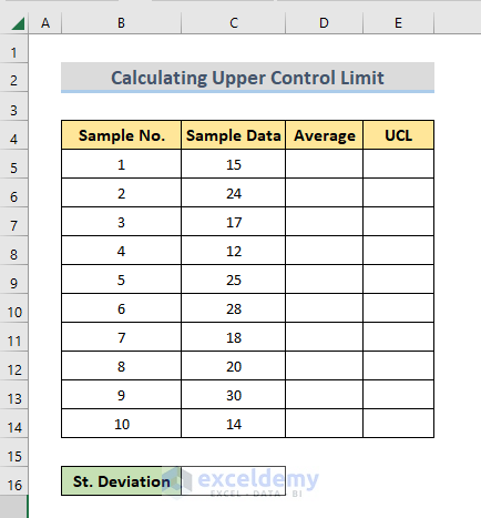
STEP 1: Input Sample Data for Upper Control Limit Calculation
- Firstly, you have to include sample data for calculating the upper control limit. For demonstration, we have included some random data in the Sample Data column.
STEP 2: Determine Average of Sample Data
- Then, we have to determine the mean of the sample data.
- To do that, we are using the AVERAGE function of Excel. Just use the following formula in Cell D5.
=AVERAGE($C$5:$C$14)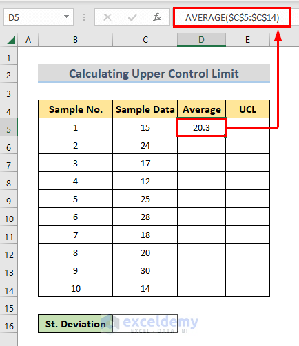
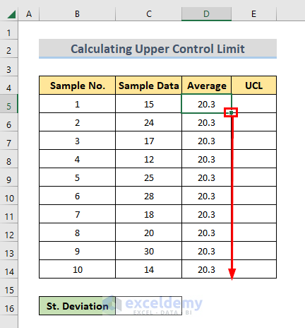
- Then, use the Fill Handle to copy the formula in the following cells.
STEP 3: Find Standard Deviation for Data
- Afterward, use the STDEV.S function to calculate the standard deviation. Just apply the following formula in Cell C16.
=STDEV.S($C$5:$C$14)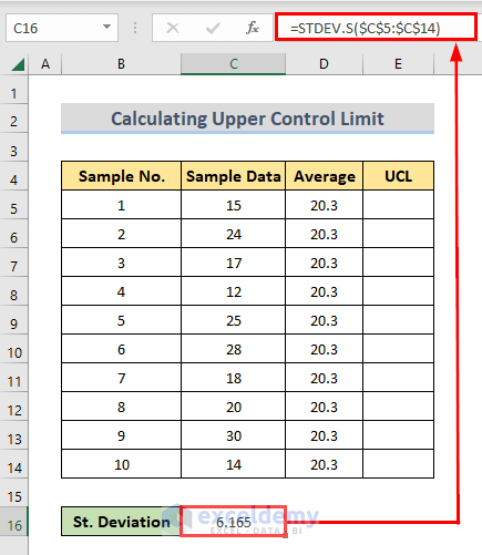
STEP 4: Calculate Upper Control Limit with Formula
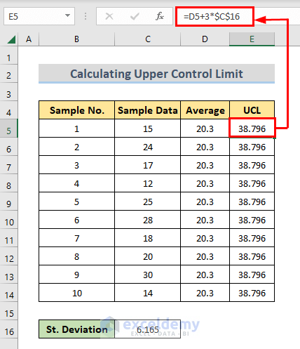
- Finally, it’s time to calculate the upper control limit.
- For that, insert the following formula in Cell E5 and press Enter.
=D5+3*$C$16- As a result, we will see the upper control limit for the sample data in Cell E5.
- At last, use the Fill Handle to copy the formula and get the UCL in the following cells.
How to Determine LCL with UCL and Create Chart with It in Excel
So far, we have calculated the upper control limit and now let’s calculate the lower control limit and make a chart with the average, upper control limit, and lower control limit. For that, follow the steps given below.
- Firstly, calculate the upper control limit following the previously mentioned procedures.
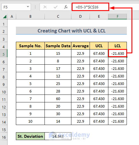
- Then, apply the following formula in Cell F5 to get a lower control limit.
=D5-3*$C$16- Afterward, copy the formula in the following cells using the Fill Handle.
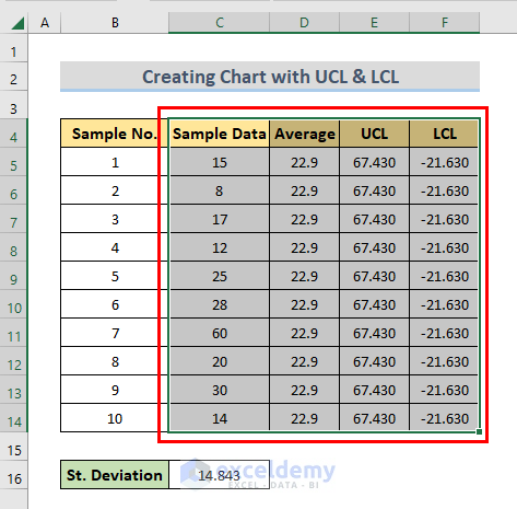
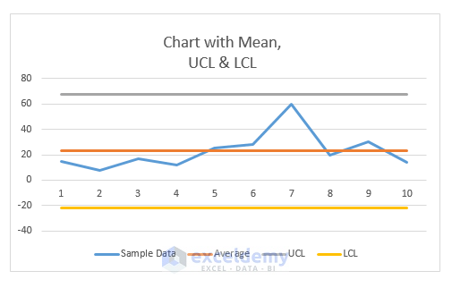
- Further, select the whole dataset including column Sample Data, Average, UCL, and LCL for creating a line chart with them.
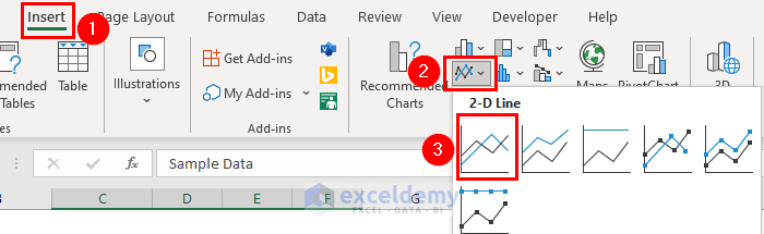
- After that, go to the Insert tab and select Line or Area Chart > 2-D > Line from the ribbon.
- Consecutively, we will see the line chart. Obviously, you can give it a suitable name.
- Later on, select any data point on the line chart and right-click on it.
- Then, select Add Data Label.
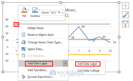
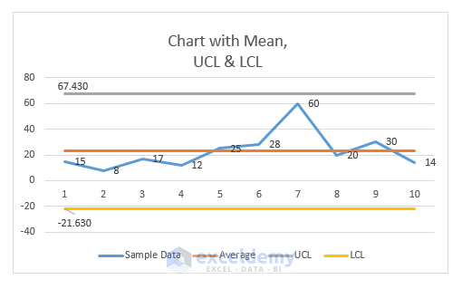
- In a similar fashion, you can add more Data Labels for a better understanding of the line chart.
Download Practice Workbook
You can download the practice workbook from here for a better understanding of the procedures.
Conclusion
Calculating the upper control limit with a formula in Excel is quite simple. Hope, you will be able to calculate the upper control limit, and lower control limit and create a line chart with them afterward. If you have any queries or suggestions, please leave a comment.
Related Articles
<< Go Back to Excel Control Chart | Excel Charts | Learn Excel
Get FREE Advanced Excel Exercises with Solutions!
