In this article, we will learn to create a progress bar based on another cell in Excel. Generally, you can’t generate a progress bar based on another cell in Excel. The progress bar appears on the cell that contains the value. But, today we will demonstrate 2 easy methods. Using these methods, you can easily create progress bars based on another cell. So, without any delay, let’s start the discussion.
How to Create Progress Bar Based on Another Cell in Excel: 2 Easy Ways
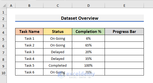
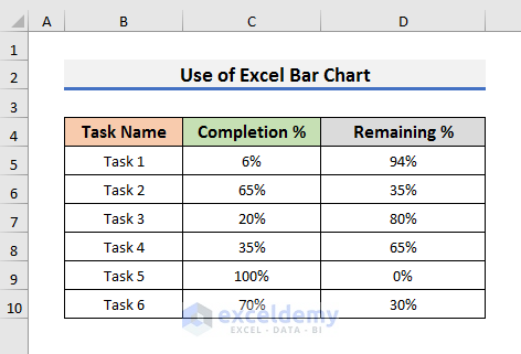
To explain the methods, we will use a dataset that contains information about some Tasks and their Completion status. In the first method, we will use Excel Bar Chart and in the second method, we will use Conditional Formatting. We will try to show the progress of each task in the progress bar.
1. Use Excel Bar Chart to Create Progress Bar Based on Another Cell
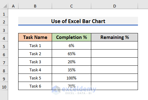
Microsoft Excel provides us with different kinds of bar charts for various purposes. We can use the 2D Stacked Bar Chart to show the progress bars of different tasks in our Excel sheet. To make the explanation easier, we have removed the Status column and also, named Column D as Remaining %. We will find out the reasons behind these changes in the following steps. So, without further ado, let’s follow the steps below.
STEPS:
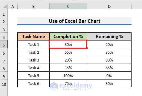
- First of all, select Cell D5 and type the formula below:
=1-C5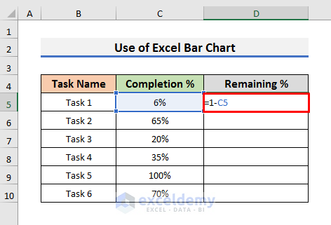
- Press Enter to see the result.
- Secondly, drag the Fill Handle down.
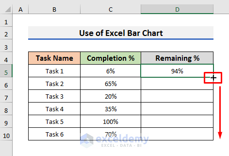
- You will see results like the picture below.
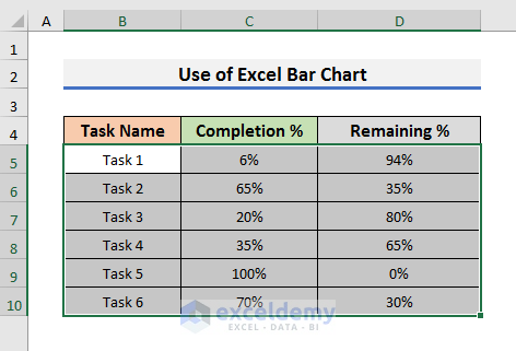
- Thirdly, select the range B5:D10 in the dataset.
- You need to select the Task Name, Completion %, and Remaining %.
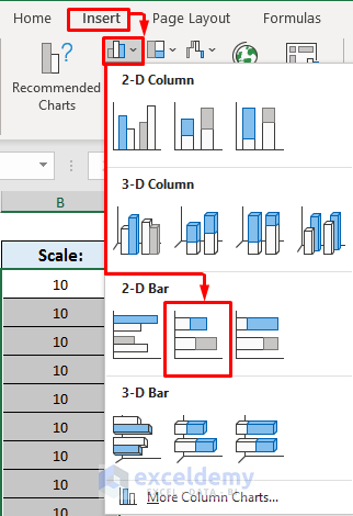
- After that, go to the Insert tab and select Bar Chart from the Charts section. A drop-down menu will appear.
- Select Stacked Bar from the 2-D Bar section.
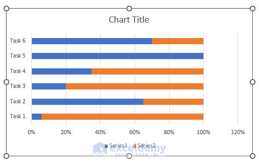
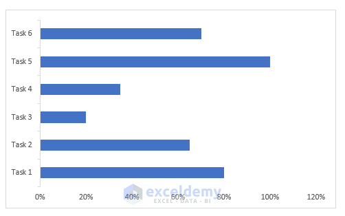
- As a result, a 2-D Bar Chart will appear on the Excel sheet.
- In the following step, click on the orange part of a bar like the picture below.
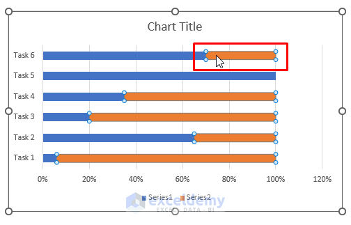
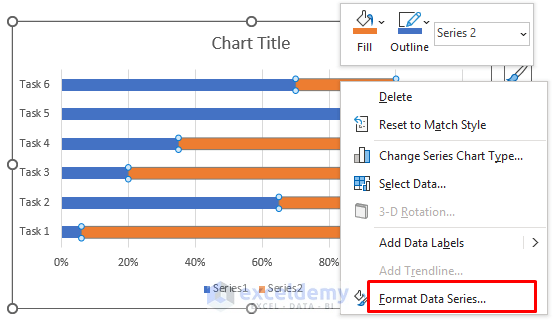
- Then, right-click on the orange part. A drop-down menu will appear.
- Select Format Data Series from there.
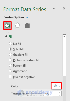
- It will open the Format Data Series settings on the right side of the sheet.
- Now, click on the Fill icon and fill the bar with a Solid White Color.
- After changing the color of the orange part to white, the progress bars will be like the one below.
- At this moment, click on the plus (+) icon and deselect Chart Title, Gridlines, and Legend.
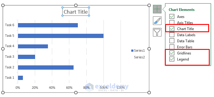
- As a result, the progress bars will look more understandable.
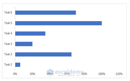
- To test the progress bars, we have changed the value of Cell C5 to 80%.
- Finally, the progress bar of Task 1 will change like the picture below.
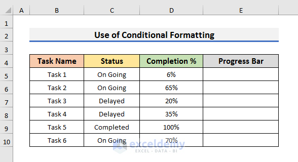
2. Make Progress Bar Based on Another Cell with Conditional Formatting
In Excel, we use Conditional Formatting according to your needs easily. Today, we will show how we can use conditional formatting to make a progress bar based on another cell. In this case, we will use our raw dataset. The steps of this method are very easy but they can be repetitive.
Let’s observe the steps below to learn more about this method.
STEPS:
- In the first place, select Cell E5 and type the formula below:
=1-D5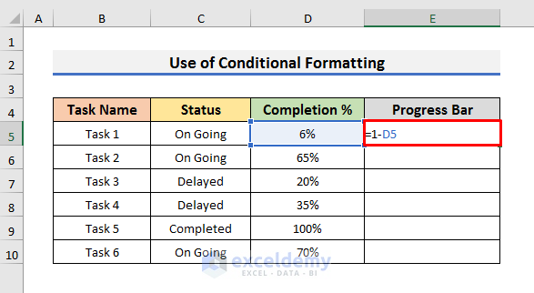
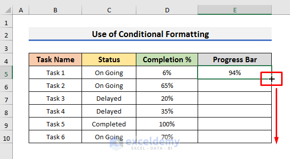
- Hit Enter to see the result.
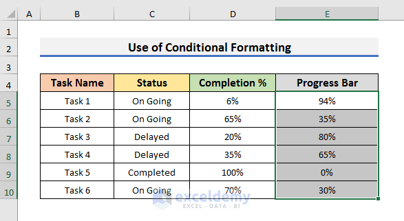
- Then, use the Fill Handle to copy the formula down.
- Secondly, select Cell E5 to E10.
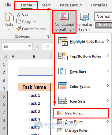
- Thirdly, navigate to the Home tab and select Conditional Formatting. A drop-down menu will appear.
- Select New Rule from there. It will open the New Formatting Rule window.

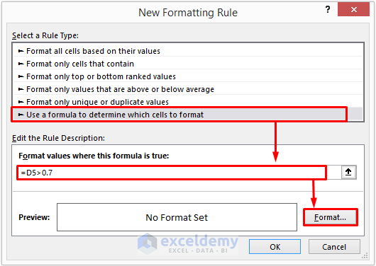
- After that, select Use a formula to determine which cells to format and type the formula below:
=D5<0.5- Then, click on Format to open the Format Cells window.
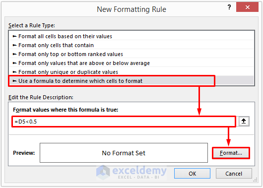
Here, the formula denotes if the value of Cell D5 is less than 50%, then, it will apply the formatting.
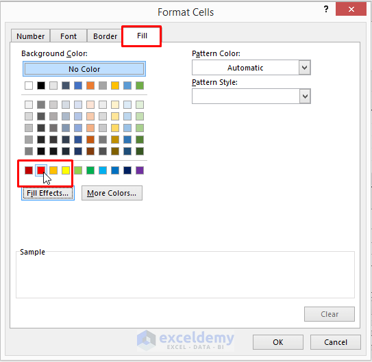
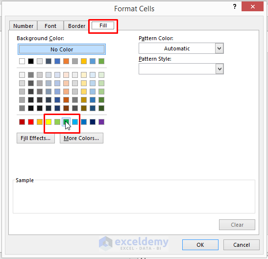
- In the Format Cells window, select Fill and choose a background color according to your choice.
- We have selected the Red color.
- Click OK to proceed.
- Again, select Cell E5 to E10.
- Then, go to the Home tab, select Conditional Formatting, and then, select New Rule.

- This time, select Use a formula to determine which cells to format but type the formula below:
=AND(D5>=0.5,D5<=0.70)- Then, click on Format.
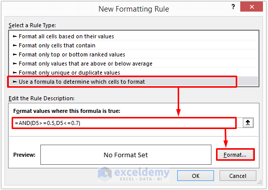
This formula indicates if the value of Cell D5 is between 50 % to 70 %, then, it will apply the formatting.
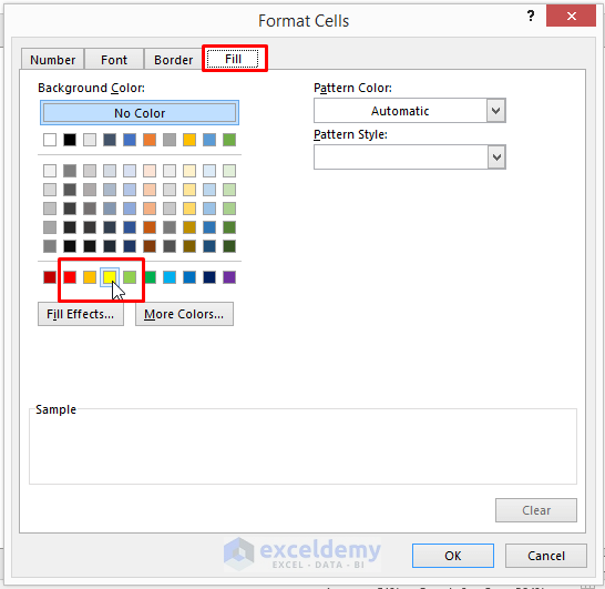
- Also, select Fill and choose Yellow as a background color in this case.
- Click OK to proceed.
- Once again, select Cell E5 to E10 and go to the Home tab, select Conditional Formatting.
- And then, select the New Rule.
- Now, select Use a formula to determine which cells to format but type the formula below:
=D5>0.70- Then, click on Format.
In this case, the formula represents if the value of Cell D5 is greater than 70 %, then, it will apply the formatting.
- At this moment, select the Green color in the Fill tab.
- Select OK to proceed.
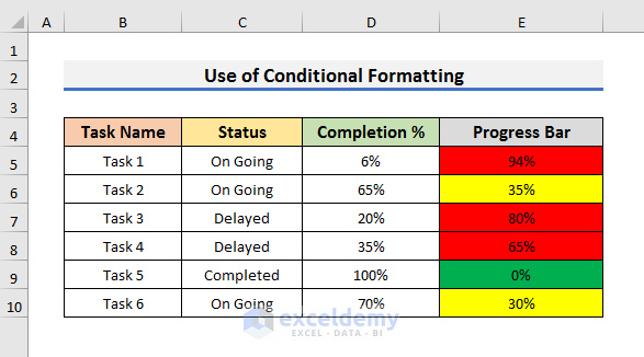
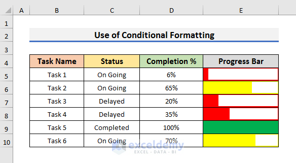
- After applying the 3 conditions, the dataset will look like the picture below.
- One last time, go to the Home tab and select Conditional Formatting.
- Select New Rule from the drop-down menu.

- Select Format cells based on their values in the Formatting Rule window.
- After that, choose Data Bar and check Show Bar Only in the Format cells based on their values section.
- Then, select Number and type 0 in the Minimum box.
- Also, select Number and type 1 in the Maximum box.
- Select Solid Fill and white color in the Bar Appearance settings.
- Most importantly, select Right-to-Left in the Bar Direction.
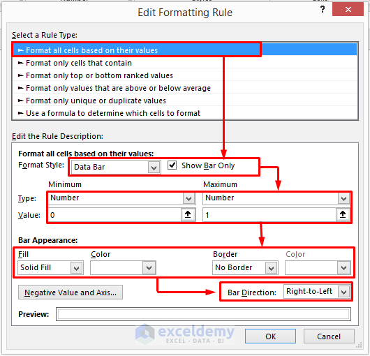
- Finally, click OK to see results like the picture below.
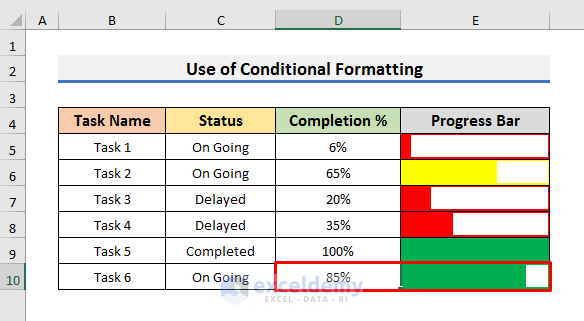
- Now, if you change the Value of Cell D5 to 85 %, the progress bar will also change according to the conditions.
Download Practice Book
You can download the practice book from here.
Conclusion
In this article, we have discussed 2 easy methods to create a Progress Bar Based on Another Cell in Excel. I hope this article will help you to perform your tasks easily. Moreover, using Method-2 you can create progress bars according to your needs. Furthermore, we have also added the practice book at the beginning of the article. To test your skills, you can download it to exercise. Last of all, if you have any suggestions or queries, feel free to ask in the comment section below.
Related Articles
<< Go Back to Progress Bar in Excel | Data Visualisation in Excel | Learn Excel
Get FREE Advanced Excel Exercises with Solutions!
