In this article, you are going to see some Excel formula symbols cheat sheet. This article will be helpful for learning about the process of inserting formulas in Excel. First of all, we are going to discuss some basic arithmetic operations of the mathematical operators. This might be helpful as most of us don’t know what the order of operations in Excel is.
The parts of Formulas will be discussed and you will also get to know about the reference and ranging of different cells in Excel.
Order and Precedence of Operators in Excel
Excel uses many symbols for mathematical operations. These mathematical operations follow some precedence. Depending upon the precedence the order of calculation is evaluated. In the below picture some operators are given along with the precedence.
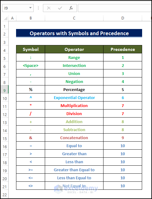
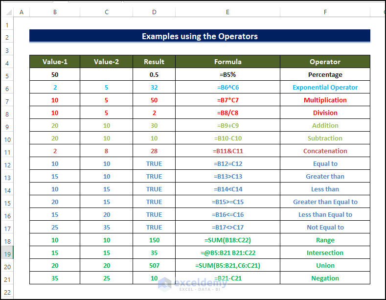
Look into the below table for a better understanding of the mathematical operations along with the results and operators.
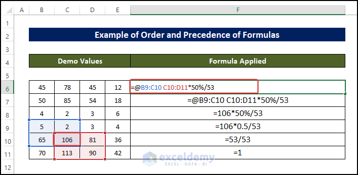
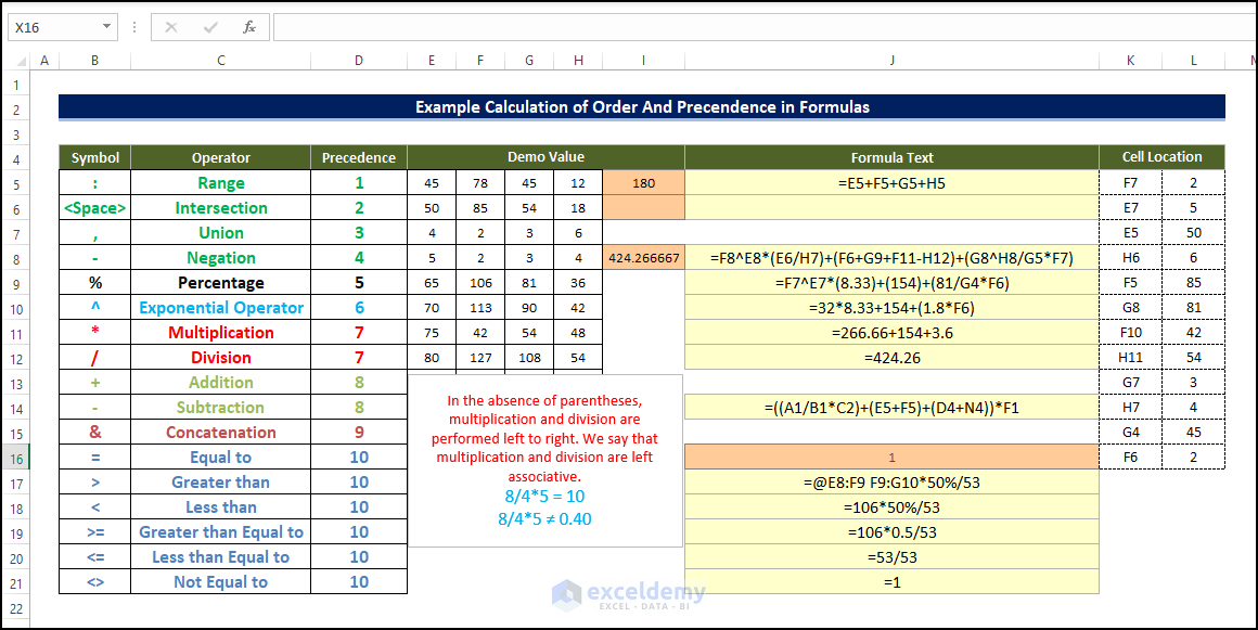
Let`s work on an example to check the order of the mathematical operations. In cell J15 we wrote =E7:F8 F8:G9*50%/53. Here the range E7: F8 selects the blue region and F8: G9 selects the red region. There is a space that we used in between the two ranges, according to the table this Space operator is used for the intersection. So, after applying the intersection between the two ranges we will get 106.
After the Range and Intersection, the operation is done the formula will calculate the Percentage. The percentage of 50 is 0.5. After that, the Multiplication and Division operations will be performed and we will get the result 1 at the end of the calculation.
Look into the below pictures where you will get more examples with the calculation process.
Basic of Excel Formulas
The formula is used to provide the expression/value of a cell. The formulas are written with an equal sign in a cell. In Excel, you can use the arithmetic sign or the built-in functions to evaluate the cell’s value. Excel Functions are the built-in formulas that are used for specific purposes. Whenever functions are used as formulas, there are arguments that are nested in between the parenthesis of functions.
Manually Entering Arithmetic Symbols as Formulas
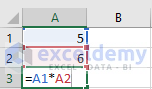
As we discussed before arithmetic signs can be used as formulas in Excel. Let`s look into an example where we will multiply two numbers. Here we will be using “*” sign for multiplying the two numbers. The numbers are located in cell A1 and in cell A2. For performing this multiplication type =A1*A2 in cell A3.
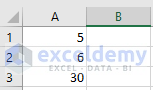
After writing the formula press on Enter and you will get the below result.
Manually Entering Functions as Formulas
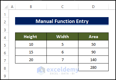
Without the functions of Excel, you cannot imagine the zest of Excel. It is kind of impossible to work without functions in Excel. There are about 400+ functions that are placed as built-in in Excel. With the upgrading of Excel`s software version, the number of functions is also growing up. To write functions as formulas first you need to assign the equal (=) sign before the function in a cell. The inputs of the functions are known as the arguments which are placed in between the parenthesis of the functions. Here we will be working on a simple SUM calculation to make yourself understand how to write the functions as formulas in Excel.
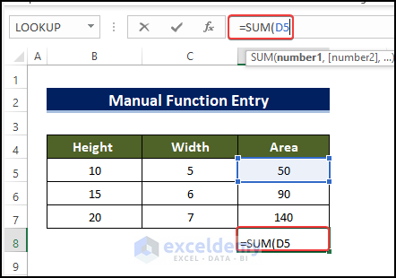
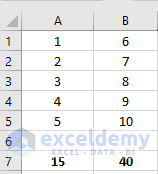
In the above picture, we calculate the sum of some numbers. The Function that is used for this calculation is SUM. In between the SUM function we gave the range of the numbers of which we want to know the sum. This range in between the Parenthesis is known as the argument. It is nothing but the input of a function. After typing the formula press on Enter to get the below result.
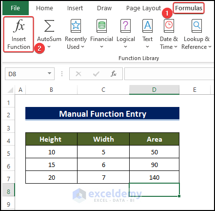
Using the Insert Function Button Option
You can use the insert button command of Excel to write formulas in a cell. In this way, you can get an idea about the functions and arguments you are using. Let`s say we want to perform the same calculation. Instead of writing the whole formula click on the cell in which you want your formula to be placed and then click on to Insert Function option under the Formulas tab.
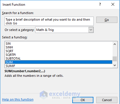
- In the Insert Function dialogue box select Math & Trig and under the Select a function drop-down menu select SUM and press OK.
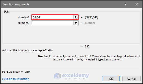
- After Selecting the SUM option, you will see it will ask for arguments to be entered. Select the range in the functions argument dialogue box.
- Enter the range of cell that need to be sum up.Press OK after this.
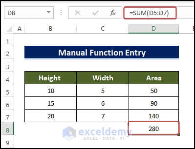
- After pressing OK, you will see that the summation of the range of cell D5:D7 is now present.
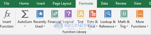
Narrowing the Search option Using the Function Library
You can use the Function Library to use the proper functions as formulas. Under the Formulas tab, you will get to see the Function Library where you can select different categories like Text, Financial, Date& Time, etc.
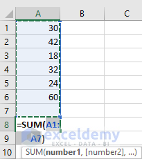
Using the AutoSum Option
The AutoSum option under the Function Library lets you performing simple calculations like sum, average, count, max, min, etc. automatically for an entire column and row. Just after the end of the column select the function that you want to use the AutoSum option. You will see it selects the range automatically.
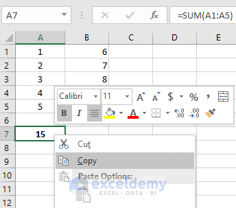
Copying and Pasting a Formula
You can easily copy a formula and paste it into different cells whenever you require them. It`s better to use the paste special option while pasting a formula. To do it, just copy the formulated cell and paste it where you want it to. In our case, we want to copy the same formula to a different column. First copy the formula.
Now use the paste option where you want to paste the formula. There are a lot of paste options. You can use the normal paste option, formula, and formatting to copy the formula.
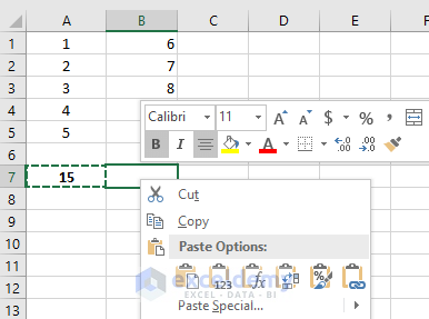
After pasting the formula, you will see that the copied formula automatically detects what to do. Like at the end of column B you wanted the formula to sum up the total column B. It automatically does that. That`s the magic of pasting a formula.
Dragging the Fill Handle
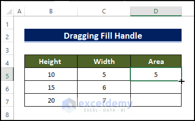
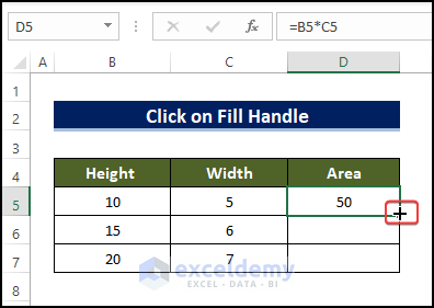
Most of the time when you use a formula in Excel, you use it for the entire row/column. The dragging of the fill handle option lets you copy this formula for the entire row and column. To do that, select the formulated cell which you want to drag. Let’s say we are calculating the area where the height and width are given in cells A2 and B2. The formula for calculating the Area is, =A2*B2. Now place this formula in cell C2 and press enter. If you select this cell C2 again you will see a green-colored box surrounds it, this box is known as the fill handle. Now drag this fill handle box downwards to paste the formula for the entire column.
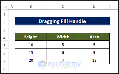
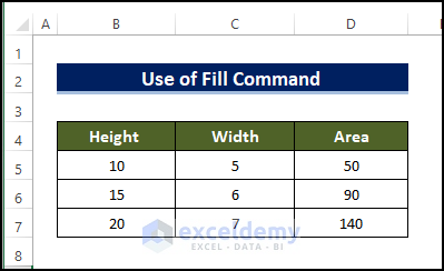
After dragging the fill handle, you will see the below result.
Double Clicking the Fill Handle
Instead of dragging the fill handle, you can double-click the fill handle option to do the same thing. Excel will automatically detect the last cell you want your formula to be copied and stop copying the formula after getting a cell with value/text in a column/row.
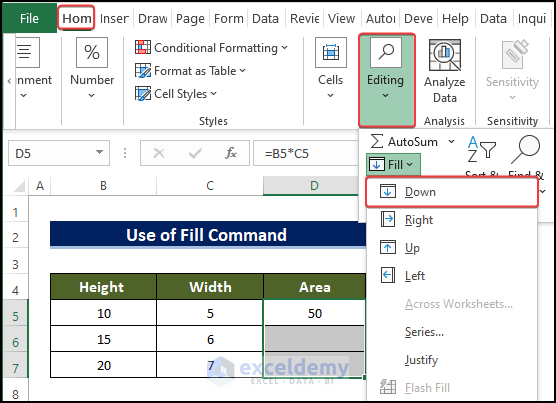
Using the Fill Option from Home Tab
You can use the Fill option from the tab to copy your specified formula either in a row or column. Under the Home Tab, select the Fill option in the Editing box. You will get to see a lot of options. To use that you need to select the cells along with the formulated cell and select the direction after clicking the Fill option from the top. In our case, we are interested to use the formula for a column so we choose the down direction.
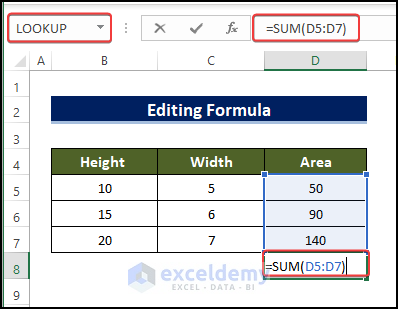
Editing a formula
Suppose you made a mistake while writing your formula. You don’t need to rewrite the formula again. Just move on to the formulated cell where you placed your formula and use backspace, delete or insert new things to edit it.
Let’s look into the below example where we had to calculate the same from the range A1: B5. We mystically gave the range A1: A5.
Now, to edit that move on to the formulated cell and double click it to edit the formula. Instead of A5 write down B5 and press on to the Enter button to get the result.
You can also use the Formula bar to edit your formulas.
Referencing Cells in Excel
You can use the “$” sign to refer cells, rows, and columns in Excel. The below table shows what are the meanings while using “$” with rows and columns.
| Symbol | Meaning |
|---|---|
| =B1 | Relative reference of cell B1 |
| =$B1 | Column absolute, Row relative |
| =B$1 | Row absolute. Column relative |
| =$B$1 | Absolute reference of cell B1 |
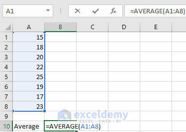
Ranging cells in Excel
To create a range in a formula, you can either write down the range manually or select the cells which will be taken as a range. Suppose, in a formula you want to know the average of some numbers located in a column of an Excel worksheet. The numbers are located from A1 to A8. You can use the formula =AVERAGE(A1: A8) for this calculation. Here A1: A8 is the range in which you are going to apply your formula. You can write it manually in the formula bar or you can select the cells by selecting them together. Look at the below picture for getting a clear idea.
Download the Working File
Conclusion
Knowing the process of inserting formulas in Excel is important. You can manually insert formula for every cell but while working on a number of columns and rows, you need to know the tricks of inserting formula in a wide range of rows and columns.
Hope you will like this article. Happy Excelling.
Related Articles
<< Go Back to Excel Tips and Tricks | Learn Excel
Get FREE Advanced Excel Exercises with Solutions!

Best article I have found yet to give the Basics. iF YOU gave a listing of all the symbols and what they mean it would be another big help.
Thank you for your public service