Sort Pivot Table by Values in Excel (4 Smart Ways)

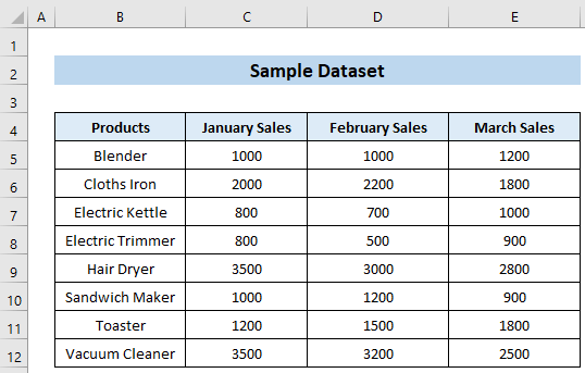
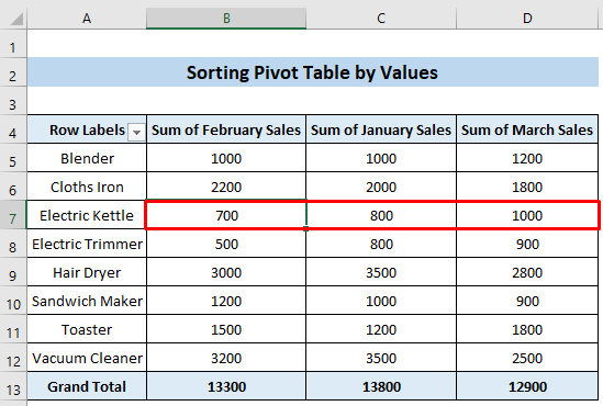
We have a dataset of different products and their respective sales for the months of January, February, and March. We have created a pivot table from this dataset and want to sort this pivot table by values.

Method 1 – Using the Pivot Table Sort Option to Sort Data by Values

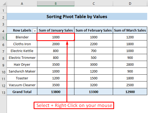
We want the January sales to be sorted in ascending order.

Steps:

• Select any cell from the Sum of January Sales column and right-click on that cell.

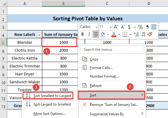
• Choose the Sort option from the context menu.
• Click on the Sort Smallest to Largest option.

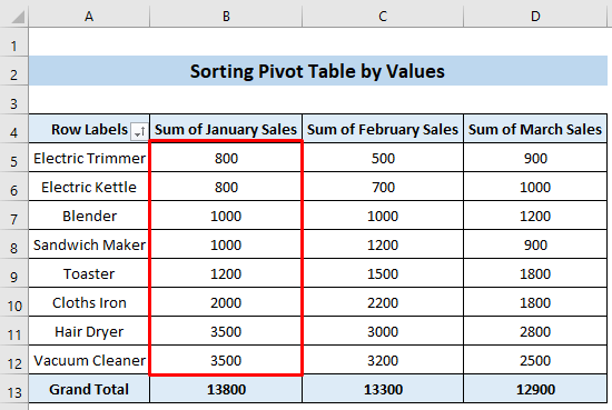
• You will sort the pivot table by January sales values in ascending order.

Method 2 – Applying the Sort & Filter Option for Sorting Values

Steps:

• Select any cell of the pivot table.
• Go to the Home tab and the Editing group.
• Click on the Sort & Filter tool and select the Sort Smallest to Largest option.

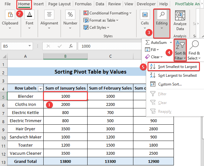
• The pivot table will be sorted in ascending order by the January sales values.

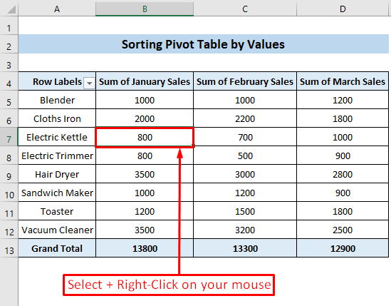
Method 3 – Using More Sort Options for Sorting a Pivot Table by Values

Steps:

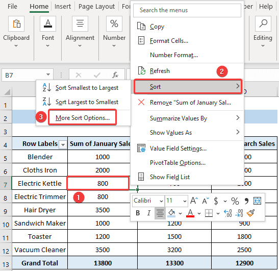
• Click on a cell inside the pivot table and right-click on it.

• Choose the Sort option from the context menu.
• Choose the More Sort Options… option.

• The Sort By Value dialogue box will appear.
• In the Sort options group, choose the Smallest to Largest option.
• In the Sort direction group, choose the Left to Right option.
• Click on the OK button.

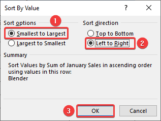
We selected the row Electric Kettle and there the lowest value was 700 which is the February Sales value for the Electric Kettle. After sorting, the number 700 will come first as it is the lowest number for the row. We will see the February Sales column now comes first due to the sorting of smallest to largest in the Electric Kettle row.

Method 4 – Applying Excel VBA Code to Sort a Pivot Table by Values

Steps:

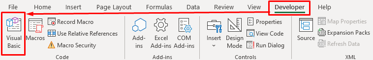
• Go to the Developer tab and select Visual Basic.

• The Microsoft Visual Basic for Applications window will appear.
• Select Sheet3 from the VBAPROJECT group and insert the following VBA code in the code window.

Sub SortPivotTableByValues()
Dim pivtbl As PivotTable
Dim pivfld As PivotField
Dim sortclm As String
sortclm = "Sum of January Sales"
On Error Resume Next
Set pivtbl = ActiveCell.PivotTable
If pivtbl Is Nothing Then Exit Sub
For Each pivfld In pivtbl.RowFields
  pivfld.AutoSort xlAscending, sortclm
Next pivfld
End Sub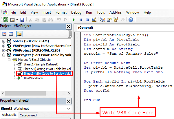

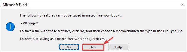
• Press Ctrl + S on your keyboard.
• A Microsoft Excel dialogue box will appear. Click on the No button.

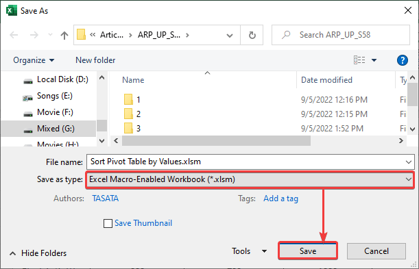
• The Save As dialogue box will appear.
• Choose the Save as type: option as .xlsm and click on the Save button.

• Close the VBA code window.
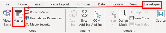
• Go to the Developer tab and select Macros.

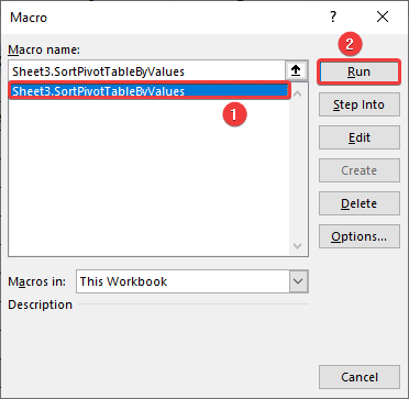
• The Macros window will appear.
• Choose the Sheet3.SortPivotTableByValues macro and click on the Run button.

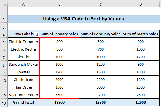
• The pivot table will be sorted in ascending order by the Sum of January Sales column.

Why Sorting the Pivot Table by Value Is Not Working

The most frequent reason is due to a custom list.

Solution:

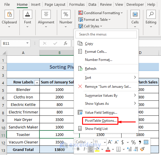
• Right-click on any cell inside the pivot table.
• Choose the PivotTable Options… from the context menu.

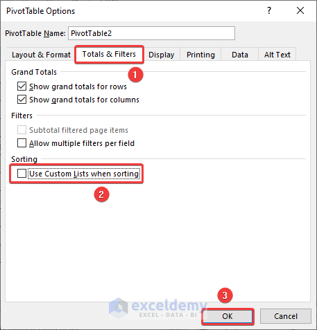
• The PivotTable Options window will appear.
• Go to the Totals & Filters tab, uncheck the option Use Custom Lists when sorting from the Sorting group, and click on the OK button.

Things to Remember

• In a pivot table, you can sort the numbers in smallest to largest or largest to smallest order.
• You can also sort alphabetical data from a to Z or from Z to A.
• If you sort a table by an individual column, the whole table will be in the sorted order of that specific column.

Download the Practice Workbook

<< Go Back to Sort a Pivot Table | Pivot Table in Excel | Learn Excel