Pivot Table Test for Interview: 6 Exercises

In this article, you will get an Excel data file for a pivot table test for an interview. There will also be six practice tasks. If you have intermediate level knowledge of Excel, you can easily solve all problems. However, the beginner can also solve a few of the problems. To solve the problems, one needs to be familiar with inserting pivot tables, using slicers, utilizing calculated fields, inserting pivot pie charts, removing the grand total, editing the pivot table, hiding the gridlines from the table, and grouping by month. If you have Excel 2010 or later, you can solve these exercises without any compatibility issues.

Download Practice Workbook

Problem Overview

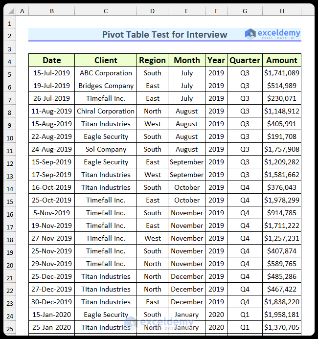
There are seven columns and 714 rows in our dataset. This represents sales data for a company from 2019 to 2022. The “Amount” column refers to the sales amount for the particular date. We’ll use this dataset to show you six exercises related to the pivot table test for an interview. The exercises are provided in the “Problem” sheet, and the solutions to those are in the “Solution” sheet. Here is a snapshot of the dataset that shows the first 21 rows of the dataset.

Let’s go through the exercises for the pivot table test for an interview.

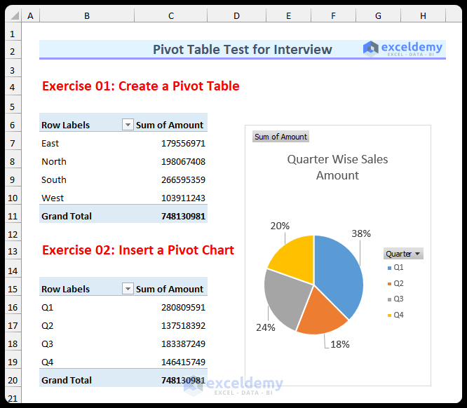
• Exercise 01: Create a Pivot Table
  • Your first task is to use the provided data to create a pivot table that displays the Zone-wise sales amount.
• Exercise 02: Insert a Pivot Chart
  • Make a pie chart with the quarterly sales data.
• Exercise 03: Group Pivot Table by Month
  • Use the Date and Amount columns to insert a pivot table. Then, group the amount by the months.
• Exercise 04: Edit Pivot Table
  • Firstly, insert a pivot table using the Client and Amount columns.
  • Then, change the column headers to “Client”, and “Sales Amount” respectively.
  • Finally, remove the Grand Total row.
• Exercise 05: Use of Calculated Field
  • Firstly, create a pivot table using the Region and Amount columns.
  • After that, Use the calculated field feature to display the tax amount for each region.
  • Here, the tax is 5% for all the regions.
• Exercise 06: Application of Slicer
  • First, insert a pivot table using the Client, Region, Year, and Amount columns.
  • Then, employ three Slicers (for Client, Region, and Year).

The animated image below shows the application of the slicers.

The following image shows the solution to the first two exercises.

Download Practice Workbook

Conclusion

Thank you for reading this article. We hope you have learned more about the pivot table test for the interview by completing these exercises. You can find more articles similar to this on the ExcelDemy website. If you have any questions or suggestions, feel free to comment below. However, remember that our website implements comment moderation. Therefore, your comment may not be instantly visible. So, have a little bit of patience, and we will solve your query as soon as possible. Keep excelling!