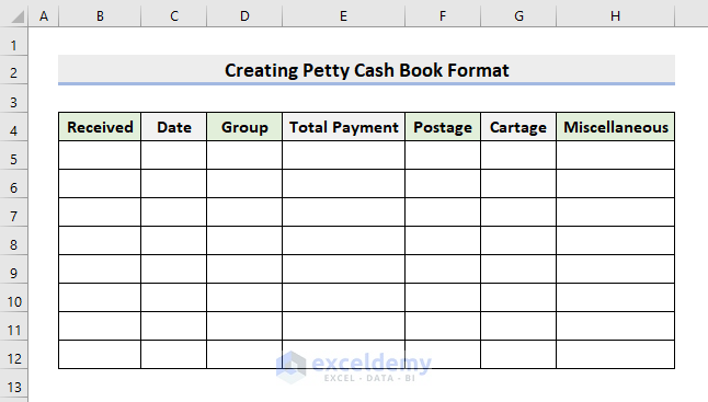
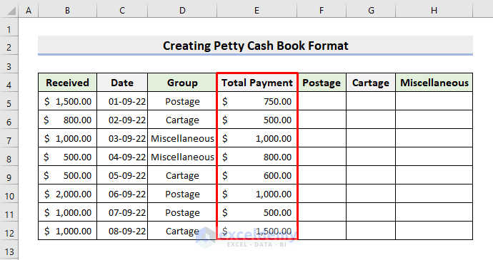
Step 1 – Design Petty Cash Book
- Input the required headers for the cash book.
- In the Received column, insert the initial amount the petty cashier will get to expend on small expenses.
- Create a Date and Group.
- The Group is about the payment type, which are Postage, Cartage, and Miscellaneous. They are also column headers.
- Another header is Total Payment on the specific date.
- You can create other headers if you need them.
Read More: How to Create Daily Cash Book Format in Excel
Step 2 – Input Received Amount & Date
- Input the received amounts and the dates. See the below picture for an example.
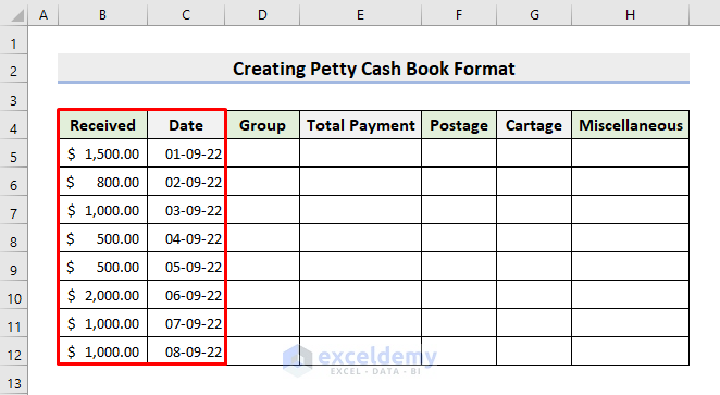
NOTE: Notice that the Received column has Accounting number format and Date has Date format in excel.
Step 3 – Fill up Group
In our example petty cash book, we have 3 types of expenses. We’ll create a drop-down list from the Group section from which you can choose instead of typing.
- Select the range D5:D12.
- Go to Data, choose Data Tools, and pick Data Validation.
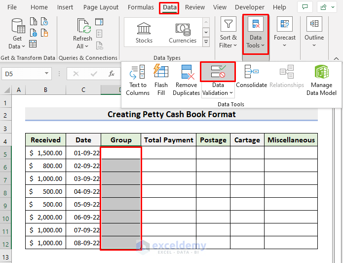
- The Data Validation dialog box will pop out. Choose Allow > List.
- Select the range F4:H4 in Source.
- Press OK.

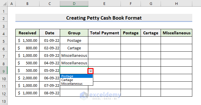
- You’ll get a drop-down symbol beside every cell in the Group column.
- You can click your desired type from there. Look at the following image for an example.
Step 4: Insert Total Payment
- Input the total payment amount manually.
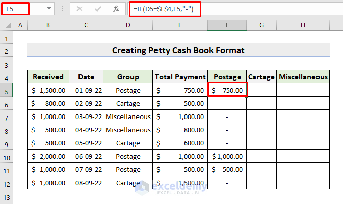
Step 5 – Create Formula for Postage
- Click cell F5.
- Copy this formula into it:
=IF(D5=$F$4,E5,"-")The IF function tests whether the D5 cell value is the same as the F4 cell value.
- Press Enter and apply AutoFill.
- The total payment amount in E5 for the postage group will be placed in this column automatically. Otherwise, it’ll be a blank cell.
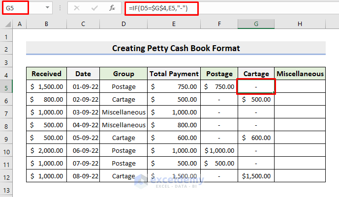
Step 6 – Apply Formula to Get Cartage
- Choose cell G5:
- Apply this formula:
=IF(D5=$G$4,E5,"-")- Hit Enter.
- Use AutoFill to complete the series.
- This returns the payment amounts for cartage.
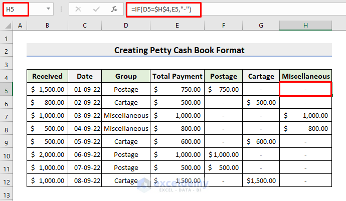
Step 7 – Generate Formula for Miscellaneous
- In cell H5, insert the formula:
=IF(D5=$H$4,E5,"-")- Pess Enter and apply AutoFill to get other outcomes.
- You’ll get expenses made for miscellaneous.
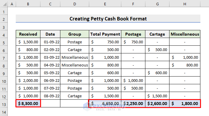
Step 8 – Calculate Total
- Select cell B13 and the range E13:H13 at the same time by pressing the Ctrl key.
- Use the AutoSum feature to get the total of Received, Total Payment, Postage, Cartage, and Miscellaneous.
- See the following picture for the result.
Step 9 – Find Present Balance
Let’s determine the book’s balance.
- Select cell F15.
- Input this formula:
=B13-E13- Click Enter.
- You’ll get the net balance.

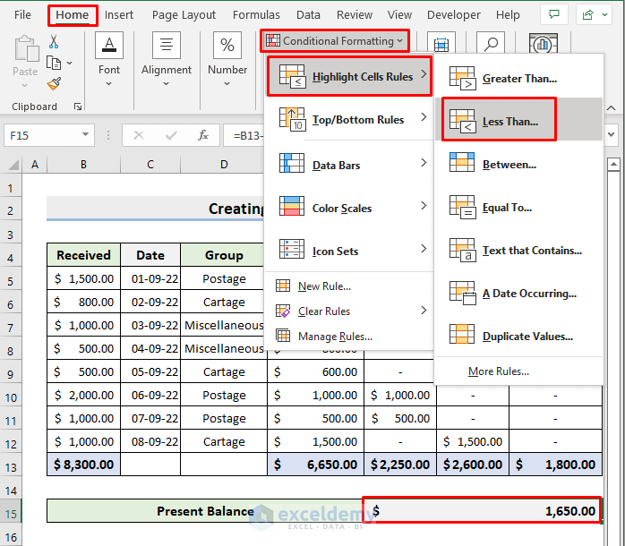
Step 10 – Apply Conditional Formatting
Let’s highlight the net balance whenever we’re running low. We’ll fill the net balance with a red color whenever it’s below $500.
- Select cell F15.
- Go to Home, click on Conditional Formatting, choose Highlight Cells Rules, and pick Less than.
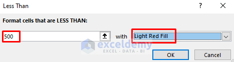
- In the pop-out dialog box, input 500 and choose Light Red Fill or any other options according to your preference.
- Press OK.
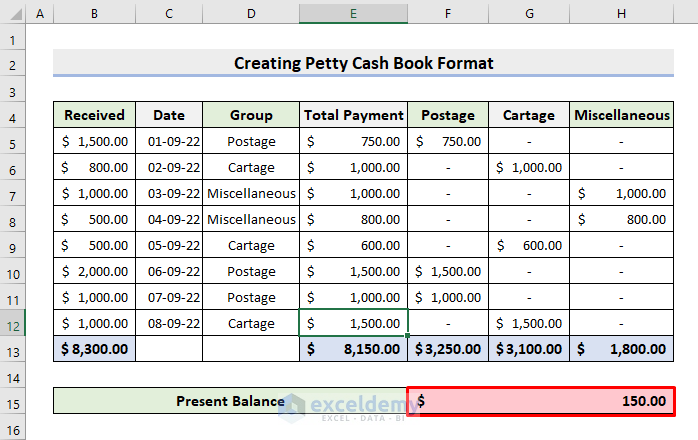
- Whenever the balance falls below $500, it’ll be filled in red as demonstrated below.
Download Practice Workbook
Download the following workbook as a template you can use.
Related Articles
<< Go Back to Excel Cash Book Templates | Accounting Templates | Excel Templates
Get FREE Advanced Excel Exercises with Solutions!
