Method-1 – Using VLOOKUP Function to Map Data in Excel
Steps:
- Navigate to the G5 cell and enter the expression below.
=VLOOKUP(G4,B5:D14,3,FALSE)
The G4 cell refers to the ID 1008, and the B5:D14 range of the cells represents the ID, Name, and Department columns.
Formula Breakdown:
- VLOOKUP(G4,B5:D14,3,FALSE) → looks for a value in the left-most column of a table and then returns a value in the same row from a column you specify. G4 ( lookup_value argument) is mapped from the B5:D14 (table_array argument) array. 3 (col_index_num argument) represents the column number of the lookup value. FALSE (range_lookup argument) refers to the Exact match of the lookup value.
- Output → Marketing
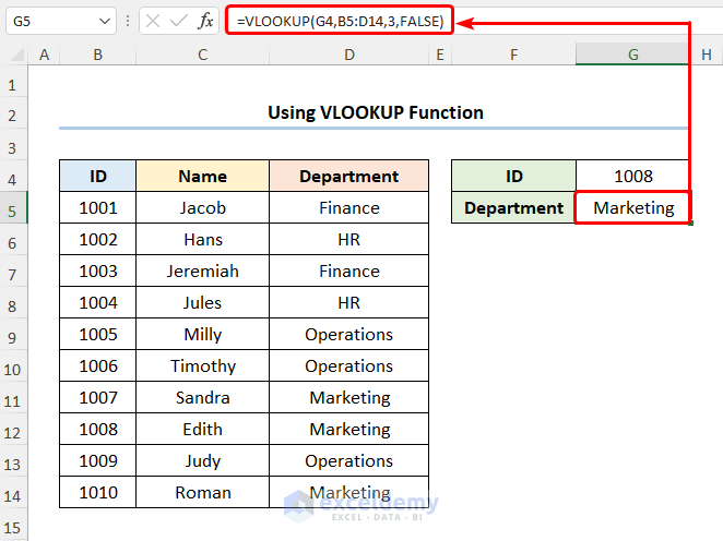
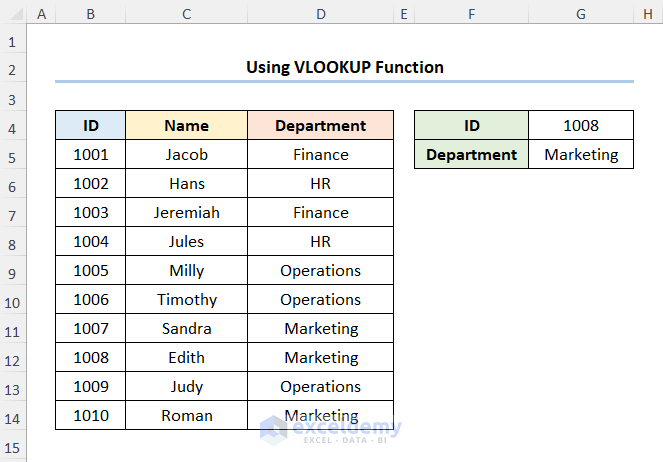
The results should look like the image given below.
Method-2 – Mapping Data with VLOOKUP and MATCH Functions (Two-way VLOOKUP)
Combine the VLOOKUP and MATCH functions to map a value at the intersection of a particular row and column. This is also known as Two-way VLOOKUP.
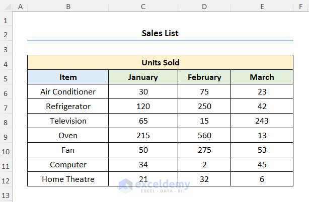
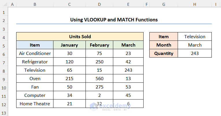
Assuming we have the Sales List dataset shown in the B4:E12 cells. We have the list of Items and the number of Units Sold in January, February, and March.
Steps:
- Select the Item and the Month, for instance, we’ve chosen Television and March.
- Go to the H6 cell and enter the formula given below.
=VLOOKUP(H4, B6:E10, MATCH(H5, B5:E5, 0), FALSE)
The H4 and H5 cells refer to the Item and Month respectively while B5:E5 represents the column headers.
Formula Breakdown:
- MATCH(H5, B5:E5, 0) → returns the relative position of an item in an array matching the given value. H5 is the lookup_value argument, which refers to the Month of March. B5:E5 represents the lookup_array argument from where the value is matched. 0 is the optional match_type argument, which indicates the Exact match criteria.
- Output → 4
- VLOOKUP(H4, B6:E10, MATCH(H5, B5:E5, 0), FALSE) → becomes
- VLOOKUP(H4, B6:E10, 4, FALSE) → H4 ( lookup_value argument) is mapped from the B6:E10 (table_array argument) array. 4 (col_index_num argument) represents the column number of the lookup value. FALSE (range_lookup argument) refers to the Exact match of the lookup value.
- Output → 243
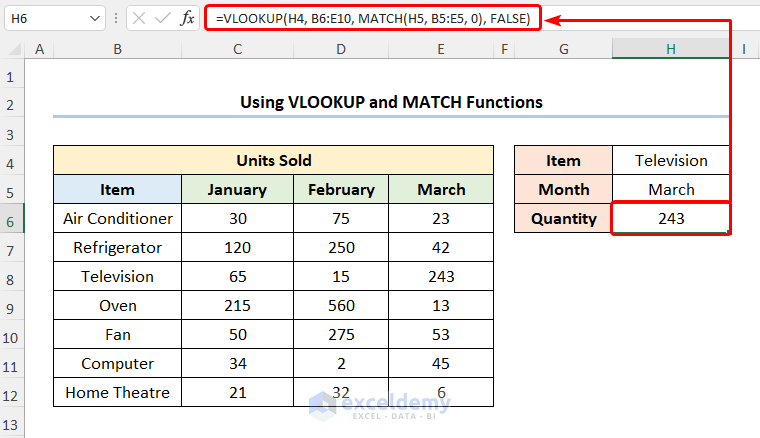
Your result should look like the picture given below.
Method-3 – Utilizing VLOOKUP and COUNTIF Functions to Map Data
Steps:
- Move to the F5 cell and enter the expression below.
=IF(COUNTIF(B5:B9,F4),VLOOKUP(F4,B5:C9,2,TRUE),0)
The B5:C9 range of cells represents the Best Seller Book and the Price columns. The F4 cell refers to the Best Seller (here, it is House of Wisdom)
Formula Breakdown:
- COUNTIF(B5:B9,F4) → counts the number of cells within a range that meet the given condition. B5:B9 is the range argument that refers to the Best Seller Books. F4 represents the criteria argument, which returns the count of the matched value.
- Output → 1
- VLOOKUP(F4,B5:C9,2,TRUE) → F4 ( lookup_value argument) is mapped from the B5:C9 (table_array argument) array. 2 (col_index_num argument) represents the column number of the lookup value. TRUE (range_lookup argument) refers to the Approximate match of the lookup value.
- Output → 25
- IF(COUNTIF(B5:B9,F4),VLOOKUP(F4,B5:C9,2,TRUE),0) → becomes
- IF(1,25,0) → checks whether a condition is met and returns one value if TRUE and another value if FALSE. 1 is the logical_test argument, which prompts the IF function to return 25 (value_if_true argument) it returns 0 (value_if_false argument).
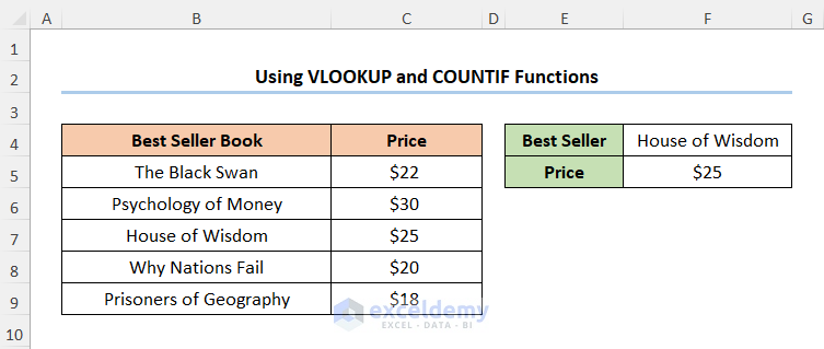
- Output → $25
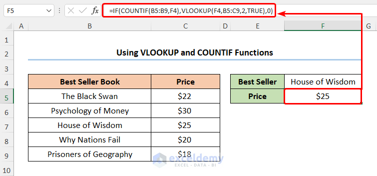
The results should look like the screenshot shown below.
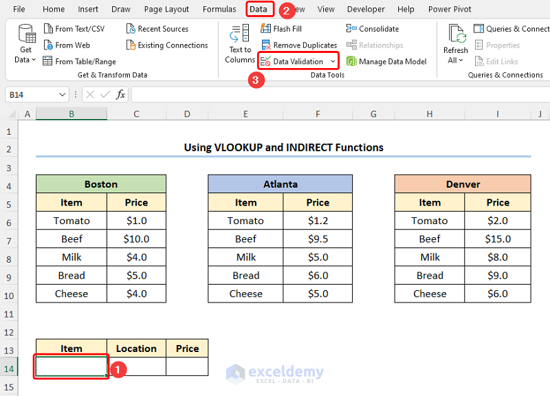
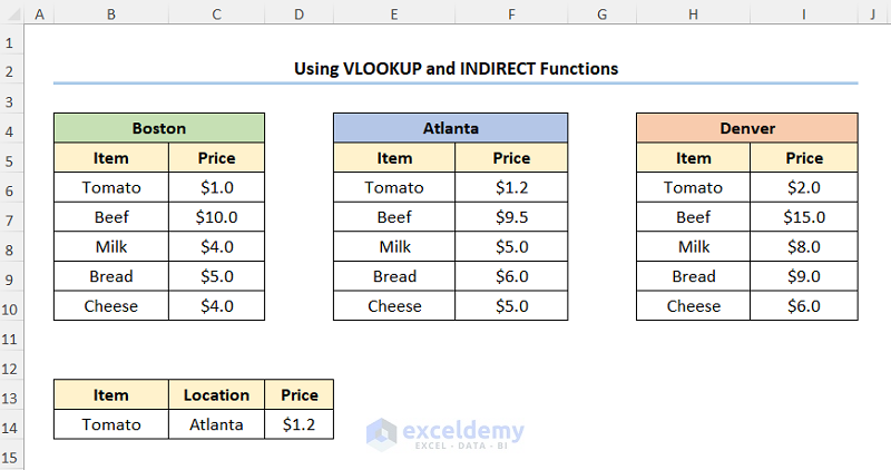
Method-4 – Mapping Data Using VLOOKUP and INDIRECT Functions in Excel
Steps:
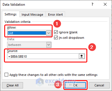
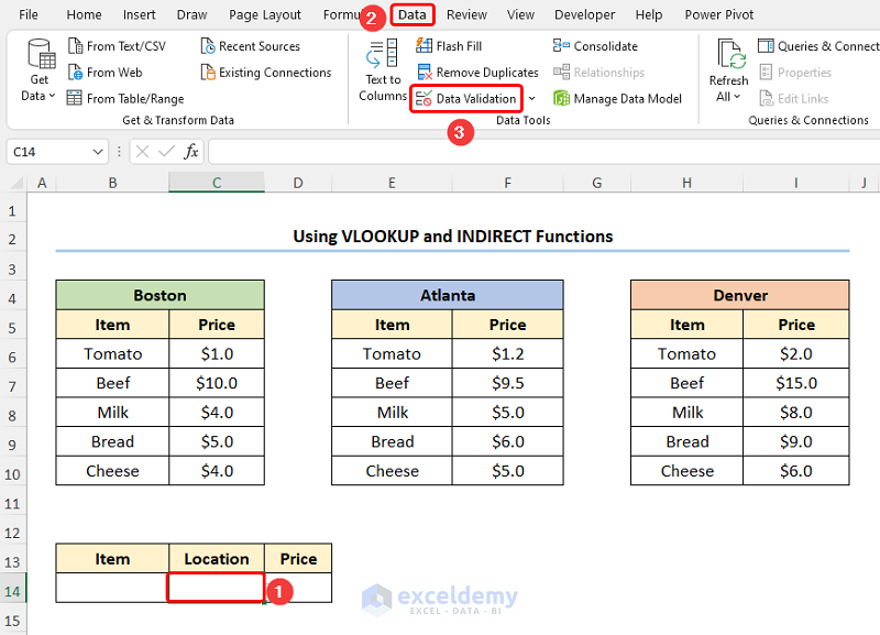
- Go to the B5 cell >> click the Data tab >> then press the Data Validation drop-down.
This opens the Data Validation dialog box.
- In the Allow drop-down, choose the List option >> in the Source field, select the B6:B10 cells >> click the OK button.
- Select the B6:C10 cells >> go to the Formulas tab >> double-click the Define Name option.
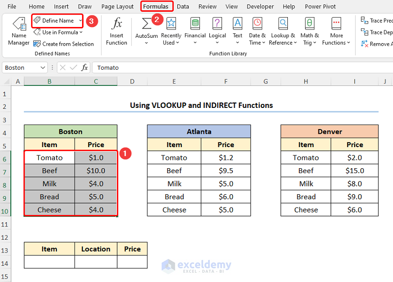
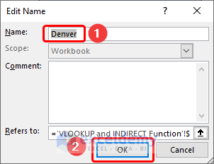
This opens the Edit Name wizard.
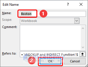
- Enter a suitable name (in this case, Boston) for the data range >> click the OK button.
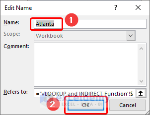
Define the Named Range for Atlanta.
Define the Named Range for Denver.
- Navigate to the C14 cell >> on the Data tab, and click the Data Validation button.
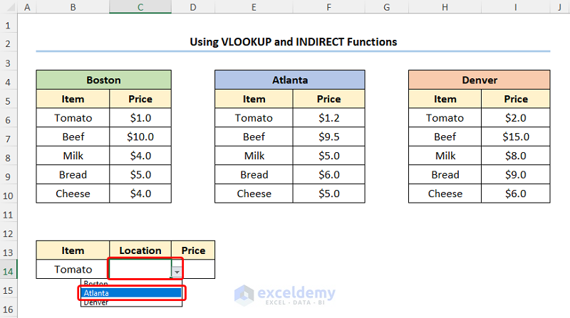
- Choose the List option >> enter the Named Ranges as shown in the screenshot below.

Choose the Item and the Location from the drop-down. We chose Tomato and Atlanta.
- In the D14 cell type in the following expression.
=VLOOKUP(B14,INDIRECT(C14),2,FALSE)
The B14 and C14 cells point to the Item and Location respectively.
Formula Breakdown:
- INDIRECT(C14) → returns the reference specified by a text string. C14 is the ref_text argument that refers to the Named Range Boston.
- VLOOKUP(B14,INDIRECT(C14),2,FALSE) → Here, B14 ( lookup_value argument) is mapped from the Named Range, INDIRECT(C14) that is the table_array argument. 2 (col_index_num argument) represents the column number of the lookup value. FALSE (range_lookup argument) refers to the Exact match of the lookup value.
- Output → $1.2
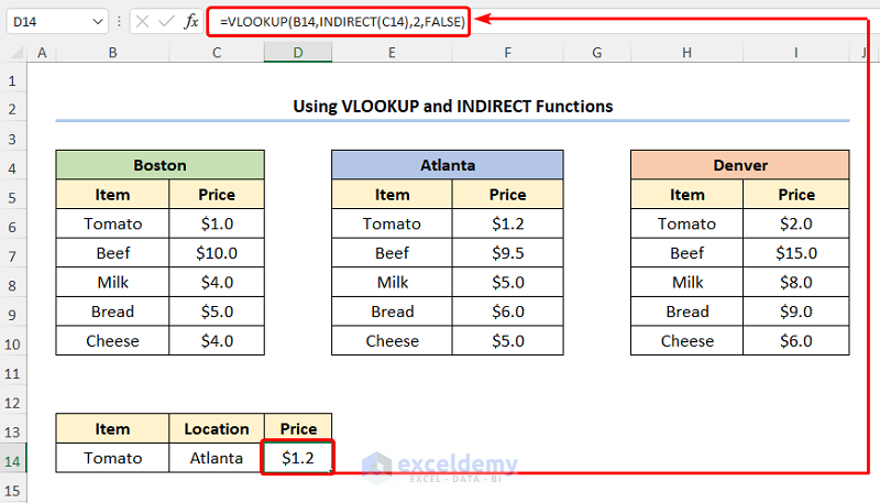
After completing the above steps the results should look like the picture below.
You may also use this method in case you want to map data from another sheet, and you want to map it from specific worksheets based on the lookup value.
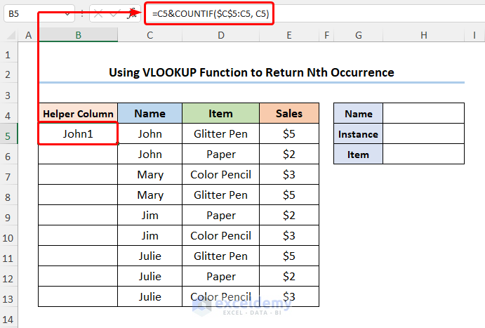
Applying VLOOKUP Function to Obtain Nth Occurrence
Steps:
- Insert a column in Column B and rename its header to Helper Column >> in the B5 cell and enter the formula given below.
=C5&COUNTIF($C$5:C5, C5)
Note: Please insert the Helper Column at the left-most side of the dataset, since, by default, the VLOOKUP function looks from left to right.
The C5 cell refers to the Name John, and the COUNTIF function counts the occurrence of John from the given range $C$5:C5. Finally, the Ampersand (&) operator combines the text and the number.
- Enter the Name and the Instance, for example, it is Julie, and 3 >> go to the H6 cell and type in the expression below.
=VLOOKUP(H4&H5, B5:E13, 3, FALSE)
The H4 and H5 cells indicate the Name and the Instance.
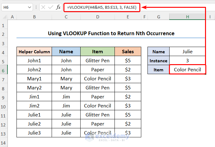
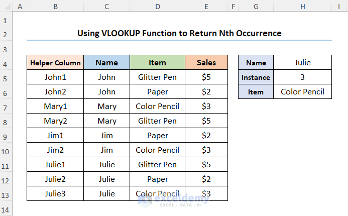
The outcome should look like the screenshot shown below.
Using VLOOKUP and IF Functions to Hide #N/A Error
Steps:
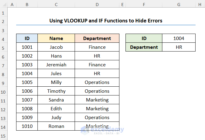
- Navigate to the G5 cell and enter the expression below.
=IF(ISNA(VLOOKUP(G4, B5:D14,3,FALSE)), "",VLOOKUP(G4, B5:D14,3,FALSE))
In this formula, the G4 cell refers to the ID 1008 and the B5:D14 range of the cells represents the ID, Name, and Department columns.
Formula Breakdown:
- ISNA(VLOOKUP(G4, B5:D14,3,FALSE)) → check whether a value is #N/A, and returns TRUE or FALSE. G4 ( lookup_value argument) is mapped from the B5:D14 (table_array argument) array. 3 (col_index_num argument) represents the column number of the lookup value. FALSE (range_lookup argument) refers to the Exact match of the lookup value.
- Output → FALSE
- IF(ISNA(VLOOKUP(G4, B5:D14,3,FALSE)), “”,VLOOKUP(G4, B5:D14,3,FALSE)) → becomes
- IF(FALSE, “”,VLOOKUP(G4, B5:D14,3,FALSE)) → checks whether a condition is met and returns one value if TRUE and another value if. FALSE is the logical_test argument which prompts the IF function to return the value from VLOOKUP function (value_if_true argument) otherwise it returns blank “” (value_if_false argument).
- Output → HR
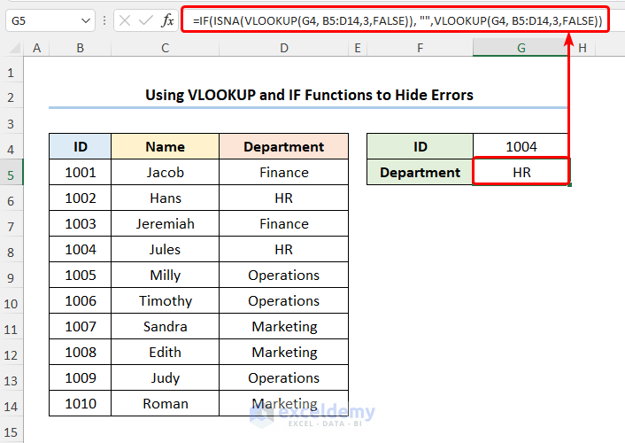
You should get the results shown in the picture below.
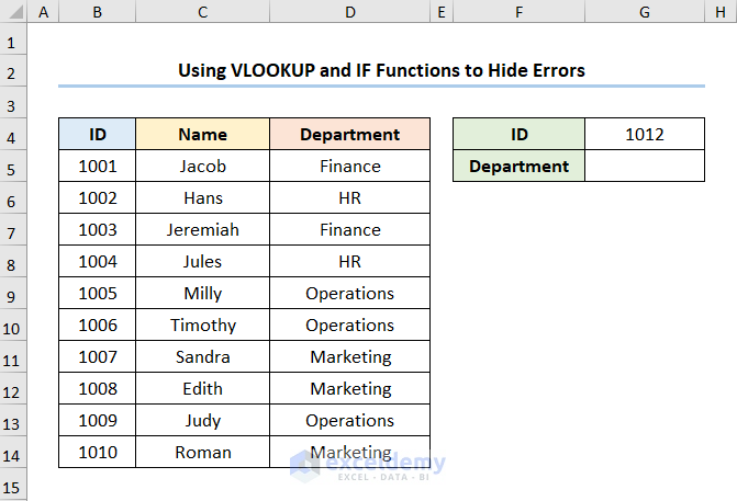
If we enter an invalid ID number (ID 1012), the formula returns a blank value instead of the #N/A error which is shown in the screenshot given below.
Download Practice Workbook
You can download the practice workbook from the link below.
Related Articles
<< Go Back To Data Mapping in Excel | Importing Data in Excel | Learn Excel
Get FREE Advanced Excel Exercises with Solutions!
