This is an overview:
The Number data type is displayed on the right side of the cells, whereas the Text data type is displayed on the left side by default.
Download Practice Workbook
What Are Excel Data Types?
There are basically two types of data in Excel:
1. Number
2. Text
Excel also offers some special types of data for geographical and stock analysis. They are available in Microsoft 365 only:
1. Stock
2. Currencies
3. Geography
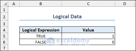
Logical data is used in formulas. The values of TRUE and FALSE are 1 and 0.
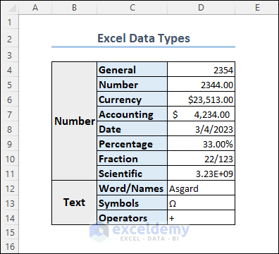
Excel Data Types – 5 Types with Practical Examples
1. Number Data
The following image shows the default Number formats available in Excel.
The largest and smallest positive numbers in Excel are 9.9e+307 and 1e-307. For negative numbers, the largest and smallest values are -1e-307 and -9.9e+307.
1.1 General
The General format is the default format of Excel data. When you type any data in an Excel cell, it will be in the General format, except for fractional numbers.
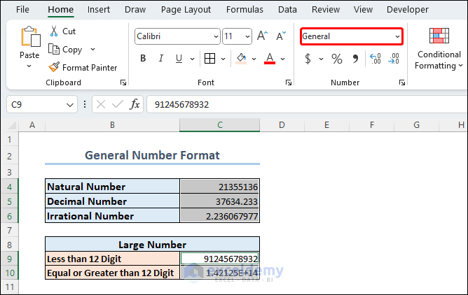
The number of decimal places in a decimal number can be anything for the General format. However, you can only see up to 10 digits of a decimal number in a cell.
If the number of digits is more than 11, you will see no change in the format. But if the number digit crosses 11, the number will automatically be converted to the Scientific format.
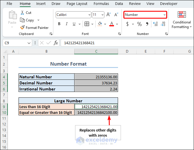
1.2 Number
The Number format shows a number by its exact or approximate value with 2 decimal places by default. If your number contains more than 15 digits, you will see 15 digits and any digit after the fifteenth is replaced with zero.
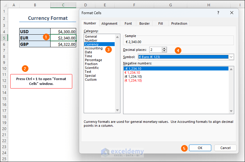
1.3 Currency
The Currency format adds the currency symbol before any number. The currency symbol is added based on the Regional Settings of your computer.
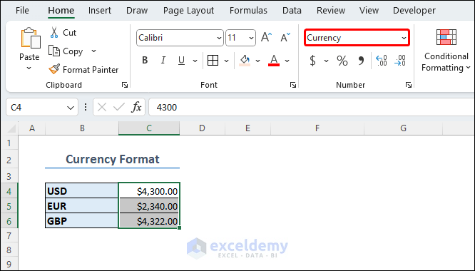
To change the currency symbol,
- Select the cell containing the number.
- Press Ctrl + 1 to open Format Cells. You can also open it in Number on the ribbon.
- Choose a currency in Currency and click OK.
This is the output.
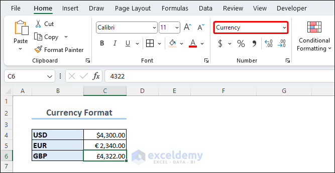
Note: The number of digits for the Currency format is similar to the Number format: you can insert a 15-digits in a cell. Any currency data that has more than 15-digits will have zeros after the 15th digit.
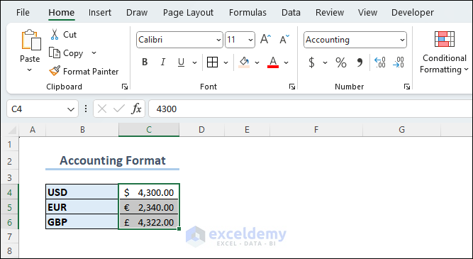
1.4 Accounting
The Accounting format is similar to the Currency format. The only difference is that the currency symbol lies on the left side of the cell while the number stays on the right.
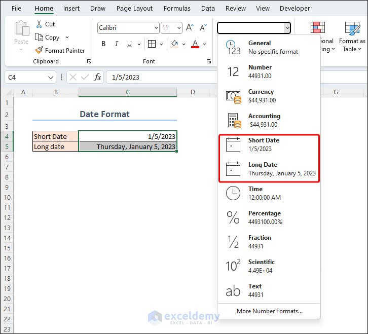
1.5 Date
By default, there are two types of date formats. They are:
- Short Date
- Long Date
The following image shows the date 5th January 2023 in these two formats.
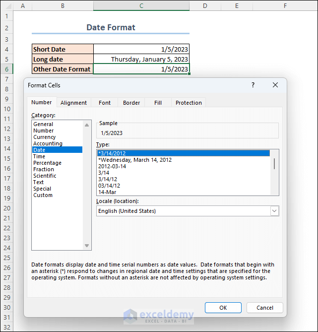
You can find more date formats in the Format Cells dialog box. Press Ctrl + 1 to open it and explore the date formats.
These are examples of commonly used date formats in Excel:
| Date Format | Description | Example |
|---|---|---|
| MM/DD/YYYY | Displays the date in the format month/day/year | 01/05/2023 |
| DD/MM/YYYY | Displays the date in the format day/month/year | 05/01/2023 |
| YYYY-MM-DD | Displays the date in the format year-month-day | 2023-01-05 |
| MMMM DD, YYYY | Displays the date in the format of month spelled out, followed by day and year | January 05, 2023 |
| DD/MMM/YYYY | Displays the date in the format of day/month abbreviated/month spelled out/year | 05/Jan/2023 |
Note:
- Choose the format that corresponds to the date conventions in your region.
- Dates are basically serial numbers starting from 1 to 2958465. 1 represents the date 1st January, 1900. Similarly, 2 and 3 represent the 2nd and 3rd days of January 1, 1900. The table below shows how Excel stores date in the serial numbers.
| Number | Date |
|---|---|
| 1 | 01/01/1900 |
| 2 | 01/02/1900 |
| 3 | 01/03/1900 |
| … | … |
| 2958465 | 12/31/9999 |
1.6 Time
Dates are serial numbers in Excel starting from the 1st of January 1900 which is stored as 1. If you insert a decimal number, Excel will return date and time formatted data. But when you select the Time format only, it will remove the date.
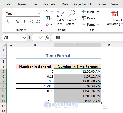
In the image above, 1.5 is converted to 12:00:00 PM (1 is stored as 1st January 1900. 0.5 is half one: half a day –12:00:00 PM).
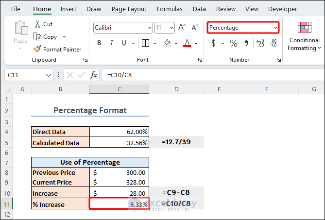
1.7 Percentage
You can also show the decimal values as percentages. The following image shows percentage formatted data.
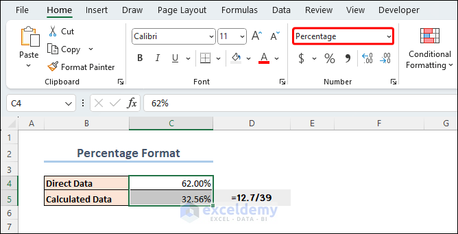
In the dataset below the previous and current prices of a product are given. To find the increment or decrement of the price in percentage, calculate the difference between the previous and current prices. Then divide the difference by the previous price. It will return a decimal value by default. Convert this decimal value to a Percentage to see the percentage increment or decrement.
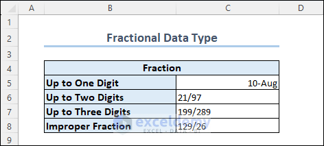
1.8 Fraction
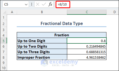
If you insert fractions in Excel without formatting, you will face issues. Excel stores “½” as 2nd January by default. If your inserted fraction matches a date, Excel will return that date. Otherwise, it returns text data.
- To solve this issue, enter an equal symbol (=) before the data and convert it to a Fraction.
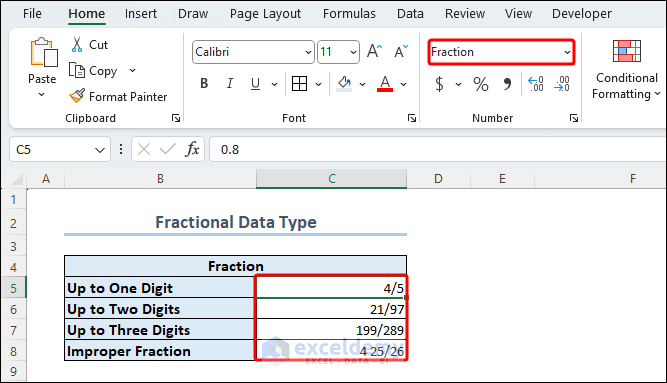
- Select the fractions and choose the Fraction format in Number.
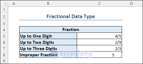
The fractions displayed are not the fractions entered: you need to change the formatting:
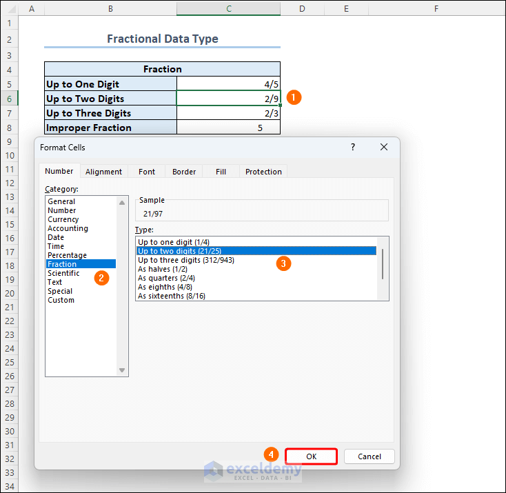
- Select the cell containing a two digit fraction and open the Format Cells window by pressing Ctrl + 1.
- Choose Fraction >> Up to two digits and click OK.
- Format three digit fractional data in C7.
This is the output.
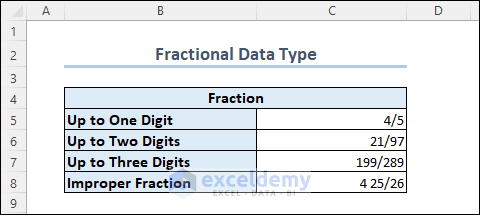
You can also convert the cell formatting to Fraction before entering fractional data.
There is no comma before data in the above image.
Note: You can also format fractional data as Halves, Quarters, Eighths etc. in Excel (see the 4th image of this section) by default. If your fraction contains a lot of digits, you need to format it using the Custom Formatting feature.
1.9 Scientific
The Scientific format shows very large or small numbers:
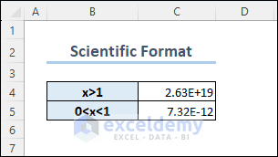
2.63E+19 is equivalent to 2.63 multiplied by 10 raised to the power of 19, which can be written as 2.63 x 10^19 or 263 x 10^17. This means that the number is 263 followed by 17 zeros: 26,300,000,000,000,000,000. However, it’s not the entered value, because the decimals taken by Excel are two approximate places by default. If you want to increase or decrease the decimal places, click Increase or Decrease Decimals in Number .
1.10 Text
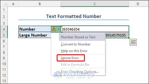
You can store data as Text. To store a large number that is not compatible with any other number format and you want to display the number as it is, you can convert the cell format to Text and enter the number:
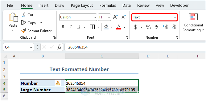
Note: Text formatted data shows the Number Stored as Text error. You can ignore it.
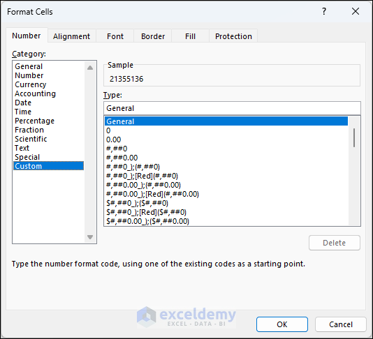
1.11 Custom Formatting Data
Customize the formatting of a cell:
- Select cells to apply the Custom option.
- Press Ctrl + 1 to open the Format Cells dialog box.
- Select Custom.
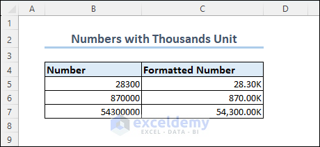
Showing Thousands and Millions Units by Formatting Cells
To show the numbers in thousands and millions:
- In Type, enter the code below to show the numbers with separators, and click OK.
#,###.00,\K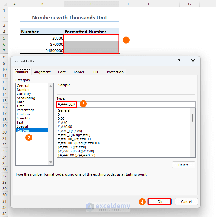
If you enter numbers in column B, you will see the Thousands format with separators.
- Use the code below to see the numbers in Millions format with separators.
#,##0.000,,\M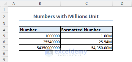
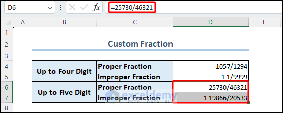
Showing Fractions
If a fraction has more than 4 digits of denominators or numerators and you want to display it in an Excel cell, use the Custom format feature.
- Use the code below for 4 digit fractions in Type of the Format Cells window.
# ####/####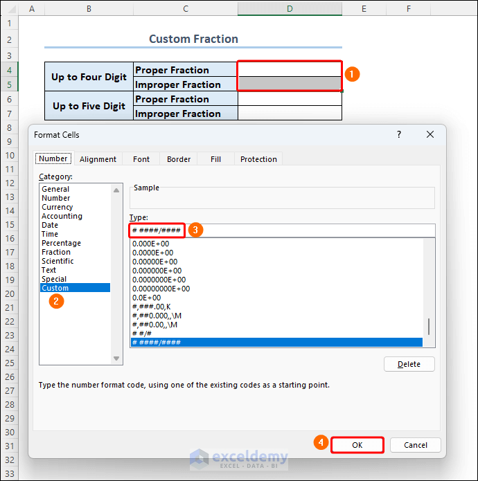
- Use # symbols to determine the number of digits in a fraction.
- Enter 4 digit fractions.
This is the output.
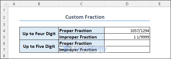
For 5 digit fractions, just add another # symbol. You may have to add an equal symbol before the fractional data if Excel stores the value as Text.
# #####/#####
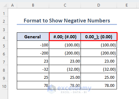
Formatting Negative Numbers
You can also format negative numbers using the following codes.
Codes:
1. #.00; (#.00)
2. 0.00_); (0.00)
1.12 Logical Data
Logical data is also numeric data in Excel. It is TRUE and FALSE. The values of TRUE and FALSE are 1 and 0 only.
These are common logical functions in Excel returning TRUE or FALSE based on the operations:
- AND: to find out whether the data meets multiple conditions.
- OR: compares values or statements that meet a condition.
- XOR: is used when only one of the data arguments can be labeled as True or False.
- NOT: filters arguments that don’t match the conditions.
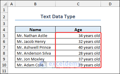
2. Text Data
Anything that is not numeric data is stored as Text data in Excel. Numeric data can also be stored as Text as described previously. section.
Text data includes alphabetical and numerical characters, and special symbols.
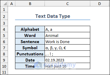
The picture above shows commonly used data types that are stored as Text in Excel.
There are no default options to format Text data but you can add texts automatically.
To add ‘Mr.’ before each name:
- Select the cell range and press Ctrl + 1 to open Format Cells.
- Select Custom and use the code below in Type.
General; General; General; "Mr. "@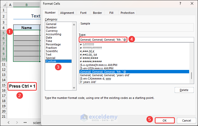
- Enter the names to see the output.
You can also add texts with numeric data.
To add ‘years old’ after the age in the dataset:
- Use the code below.
0 "years old"- Enter the ages to see output.
Note: Age data is numeric and can be used for calculation purposes.
3. Compound Data
Compound data refers to mathematical functions.
A function was created to calculate the multiplication of two numbers divided by two. The LAMBDA function can be used to create this custom function. The numeric value of the Compound data is 128. The TYPE function shows how Excel identifies Compound data with this numeric value.
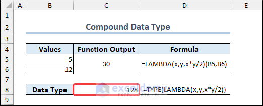
Note: The LAMBDA function can be used to create custom functions without the help of VBA.
4. Error Data
If Excel identifies data mismatch, improper function application, or any kind of malfunction in the sheet, it returns Error data. For example, if you add text to numeric data, Excel will return a #VALUE! Error:
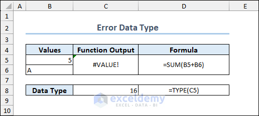
5 was added to A, which is not a compatible calculation. The numeric value for the error data type is 16.
These are common errors:
- #VALUE!: a calculation has one or more cells with incorrect data type or an incompatible operation.
- #REF!: If you remove or paste data in a cell or range of cells where you previously input a formula, an invalid cell reference error value may result.
- #N/A: there is no value available for the function to calculate.
- #NUM!: If you enter an invalid formula or function, a #NUM! value may show. It may also occur if the total produced by a formula or function is too large for Excel to display in a cell.
- #NAME?: If you have a value inside a formula without quotations or with a missing beginning or end quote, you may see this value. It may also happen if there is an error in the formula.
- #DIV/0: If you attempt to divide an integer by zero, Excel displays #DIV/0.
- #NULL!: When you insert an erroneous range reference in a formula, Excel displays the #NULL! error.
5. Excel Linked Data Types (Special Features)
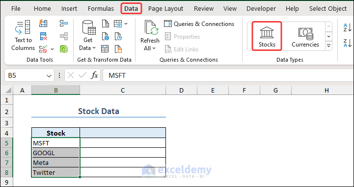
5.1 Stock Data Type
- To operate with Stock data, enter the keywords or full names of the companies.
- Select the company name range and go to Data >> Stock in Data Types.
The selected companies will be converted to Stock. You can access a lot of information about the companies by clicking the icon marked 2 in the image below.
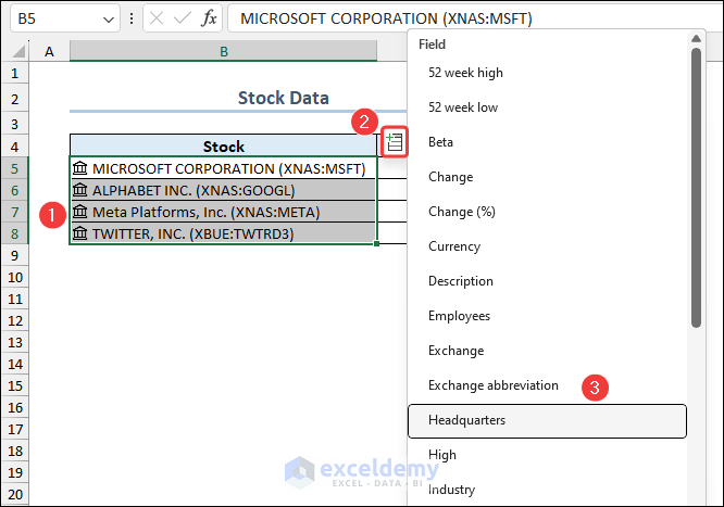
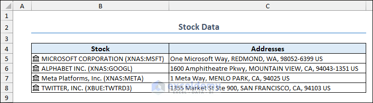
Here, the Headquarters of the Stock companies.
5.2 Currencies Data Type
To know the currency amount of Euro against 1 US Dollar:
- Enter “USD/EUR” or “USD:EUR” in a cell and select Currencies Data Type for this cell.
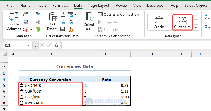
The image above displays currency rates.
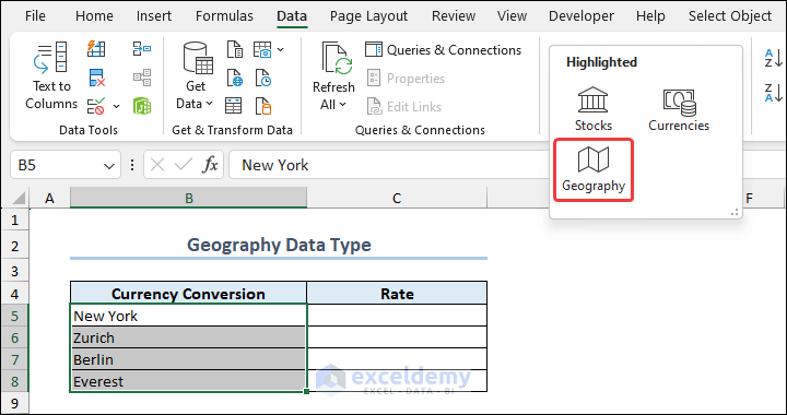
5.3 Geography Data Type
The following image shows how to apply this feature to selected cells.
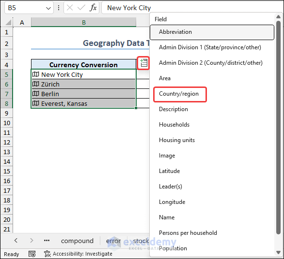
The above places are converted to Geography data. If you click the icon marked below, you will see several fields about the place: Area, Country, Population, Longitude, Latitude etc.
- To know the regions of these places, select Country/region.
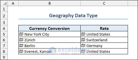
This is the output.
How to Create Data Types in Excel
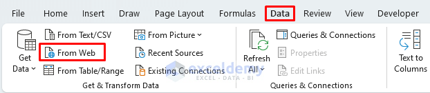
To create a list of the top scorers of the UEFA Champions League:
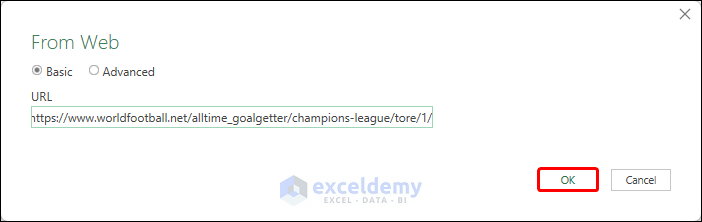
- Select Data >> From Web.
- In the From Web window, insert a link that has the list of top scorers of UCl.
- Click OK.
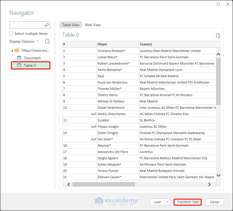
The tables available on the website will be shown as a preview in the Navigator Search.
- Click Transform Data. Here, Table 0 contains the list of players.
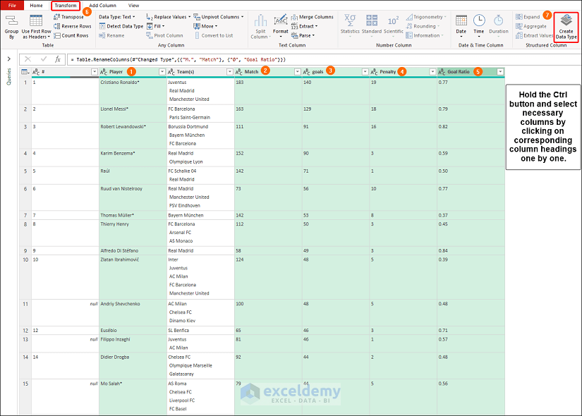
The table will be displayed in the Power Query Editor.
- Select the column heading of the column that you want to appear first in the linked data.
- Hold Ctrl and select other column headings. Here, 1 to 5.
- Select Transform >> Create Data Type.
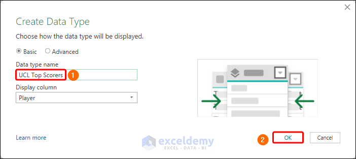
- In the Create Data Type window, name this Data Type and click OK.
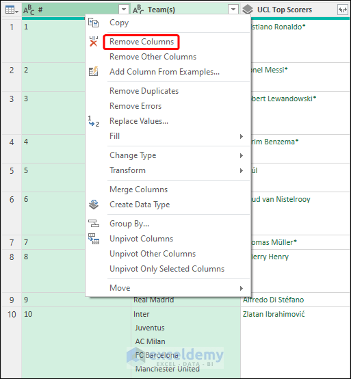
- Select unnecessary columns, right-click any of them and remove them by selecting Remove Columns.
- Select Home >> Close & Load.

The linked data type will appear in a new sheet.
- Click the icon marked as 1 and you will see the fields selected earlier in the Power Query Editor. Choose goals.
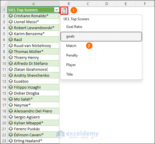
The goals different players scored will be displayed.
Excel Data Types are Missing – Solutions
Data types may not be seen in the Data tab.
1. Restart the PC
Sometimes, Excel files can be bugged and Data Types can be missing. Restarting the PC can be the primary solution to this issue.
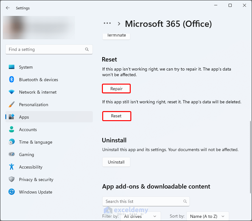
2. Repair Or Reset Excel 365
Most issues can be fixed by reinstalling the Office apps.
- Press Windows + I to open Settings.
- Select Apps >> Installed Apps.

- In the Office app, click the dotted icon marked 2 in the picture below.
- Select Advanced options.

- Choose Repair or Reset. If you want the Excel app data unchanged or intact, repair the app. If that doesn’t work, reset it. Resetting will remove your app data.
How to Check Data Type in Excel
The table shows the numeric values for all data types.
| Data Type | TYPE Function Output |
|---|---|
| Number | 1 |
| Text | 2 |
| Logical value | 4 |
| Error value | 16 |
| Array | 64 |
| Compound data | 128 |
Length of Different Numeric Data Type in Excel
The following table shows the size of different numeric data in bytes in Excel.
| Data Type | Size (Byte) | Description |
|---|---|---|
| Byte | 1 | A number ranging from 0 to 255 that is used to store binary data. |
| Integer | 2 | Integer from -32,768 to 32,767. |
| Long | 4 | Integer from -2,147,483,648 to 2,147,483,647 |
| Single | 4 | Float precision to 6 decimal places |
| Double | 8 | Float precision with double precision |
| Decimal | 14 | Fixed precision and scale (precision up to 28). |
| Boolean | 2 | Logical value (TRUE/FALSE) |
| String | Text object. Flexible length or 64 kilobytes. | |
| Object | 4 | Reference to an object. |
| Date | 8 | Date Range: 1/1/100 to 12/31/9999 |
| Currency | 8 | A number with fixed 4 decimal places |
| Variant | 16 | Special values such as Null, numeric value, text, reference to the object or variable array. |
Things to Remember
- Depending on the context, Excel may automatically transform data from one type to another.
- Different Excel formulas and functions have different data type requirements.
- Excel may treat numbers and text differently when sorting or filtering data. Text values are normally sorted alphabetically, while numerical values are often sorted in ascending or descending order.
- Mind data types in the source and destination when importing data into Excel or exporting it to other apps. Ensure data types are compatible and appropriately mapped.
Frequently Asked Questions
1. How can I identify and handle errors in Excel data types?
Answer: Use error-handling functions such as IFERROR, ISERROR, or ISERR.
2. What type of files are supported in Excel?
These files are compatible with Excel:
- Excel Workbook (.xlsx)
- Excel Macro-Enabled Workbook (.xlsm)
- Excel Binary Workbook (.xlsb)
- Template (.xltx)
- Template (Code; .xltm)
- Excel 97- Excel 2003 Workbook (.xls)
- Excel 97- Excel 2003 Template (.xlt)
- Microsoft Excel 5.0/95 Workbook (.xls)
- XML Spreadsheet 2003 (.xml)
- XML Data (.xml)
- Excel Add-In (.xlam)
- Excel 97-2003 Add-In (.xla)
- Excel 4.0 Workbook (.xlw)
- Works 6.0-9.0 spreadsheet (.xlr)
Related Articles
- How to Enable Editing in Excel
- How to Press Enter in Excel Without Changing Cells
- Making Same Change to Multiple Worksheets in Excel
<< Go Back to Learn Excel
Get FREE Advanced Excel Exercises with Solutions!
