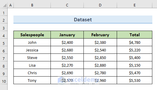
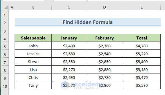
The sample dataset consists of sales of six salespeople in January and February. We can see the total sales in another column. We’ll hide the formulas.
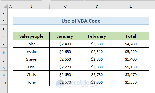
Method 1 – Using VBA Code to Hide Formulas in Excel without Protecting the Sheet
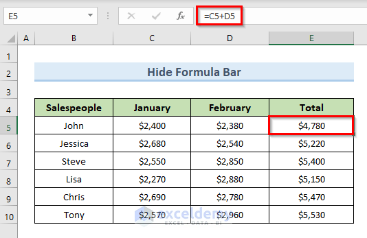
We will use the following dataset.
- If we click on cell E5, we can see the following formula in the formula bar:
=C5+D5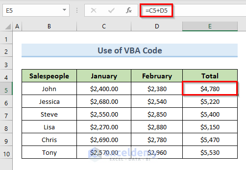
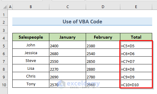
- Users can see the formulas of the following image in the formula bar just by clicking on that cell.
STEPS:
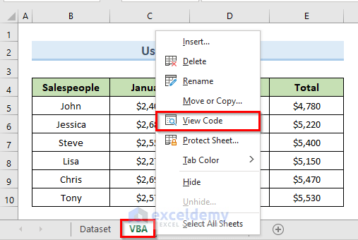
- Right-click on the sheet name.
- Select the option View Code.
- This will open a blank VBA module.
- Insert the following code in the blank VBA module:
Dim zDic As New Dictionary
Private Sub Worksheet_SelectionChange(ByVal Target As Range)
Dim zCell As Range
Dim zRg As Range
Set zRg = Range("E5:E10")
If zDic.Count <> zRg.Count Then
For Each zCell In zRg
zDic.Add zCell.Address, zCell.FormulaR1C1
Next
End If
If (Target.Count = 1) And (Not Application.Intersect(zRg, Target) Is Nothing) And (Target.HasFormula) Then
With Target
.Value = .Value
End With
Else
For Each zCell In zRg
zCell.Formula = zDic.Item(zCell.Address)
Next
End If
End Sub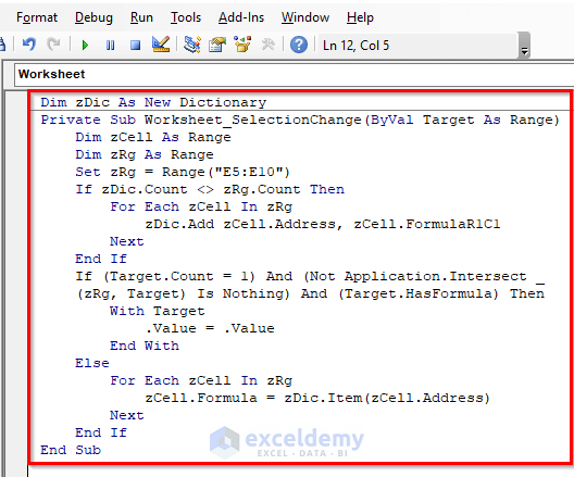
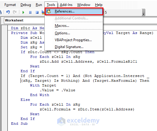
- Go to Tools and click References.
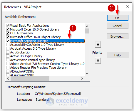
- A new dialog box named References – VBAProject will appear.
- Check the Microsoft Scripting Runtime box from the Available References section.
- Click on OK.
- Press Alt + Q to close the VBA module.
- Click on cell E5. The formula bar is showing only the value instead of the formula.
Method 2 – Hiding the Excel Formula Bar to Conceal Formulas Without Protecting the Sheet
If we select cell E5, the formula of that cell becomes visible in the formula bar.
STEPS:
- Go to the File tab.
- Select Options.

- You’ll get Excel Options.
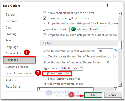
- Select the Advanced tab.
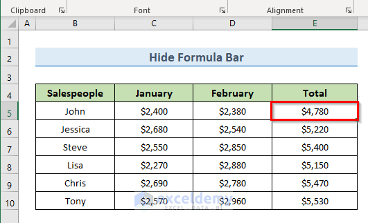
- Uncheck the Show formula bar box from the Display section and click on OK.
- The formula bar disappears from the ribbon. If we select any cell that contains a formula, the formula will not appear in the formula bar.
Read More: Hide Formulas and Display Values in Excel
Find Cells with Formulas in Excel
In the following dataset, we will determine which cells contain formulas.
STEPS:
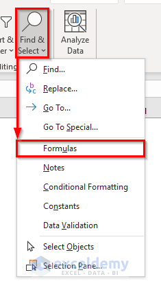
- Go to the Home tab.
- Select the option Find & Select from the Excel ribbon.
- Select the option Formulas from the drop-down menu.
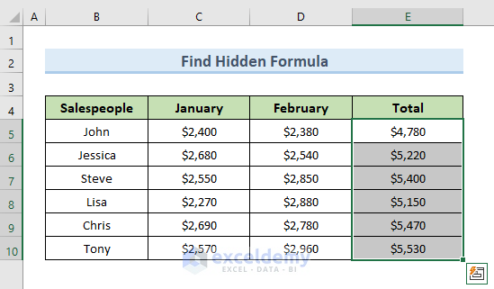
- The cells (E5:E10) that contain formulas are selected in our dataset.
Download the Practice Workbook
Related Articles
<< Go Back to Hide Excel Formulas | Excel Formulas | Learn Excel
Get FREE Advanced Excel Exercises with Solutions!

I am a beginner to learn excel VBA. I’ve just started and I am so lucky to have found this great site. Thank you and please keep going.
About the method of hiding formula without protecting sheets. I followed and it worked.
However, when I click on the cell with the formula hidden, I still see the formula for a blink before it is converted to a value. Furthermore, if I click and hold the mouse on that cell, the formula is displayed as normal until I release the mouse pointer.
Can you please update the code to fix this?
Thank you so so much.
Hello Ruby,
Thanks for your query. If you do not want to see the formula for a blink then you have to do it by protecting the worksheet. You can try the following code:
Sub HideFormulasDisplayValues()
With ActiveSheet
.Unprotect
.Cells.Locked = False
.Cells.SpecialCells(xlCellTypeFormulas).Locked = True
.Cells.SpecialCells(xlCellTypeFormulas).FormulaHidden = True
.Protect AllowDeletingRows:=True
End With
End Sub
that was great dear,love it.
Hello Matthew,
Thanks for your feedback and appreciation. Glad to hear that you loved our article. We always try to come up great topics and articles. Keep Excel-ing with ExcelDemy!
Regards
ExcelDemy