Dataset Overview
We have a simple dataset where we need to group data.
Step 1 – Create an Excel Table
- Select any cell within your dataset.
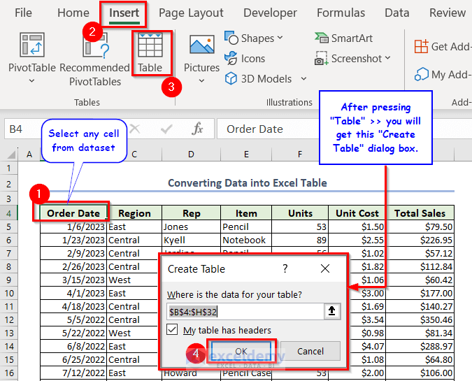
- Go to the Insert tab and click on Table.
- In the Create Table dialog box, ensure that the Where is the data for your table? box is automatically filled (based on your selection).
- Confirm that My table has headers is checked.
- Press OK to create the Excel table
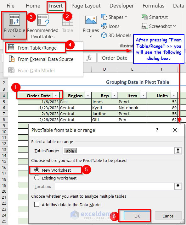
Step 2 – Generate a Pivot Table from the Excel Table
- Once you have the Excel table, select any cell within it.
- Go to the Insert tab again, and this time choose PivotTable > From Table/Range.
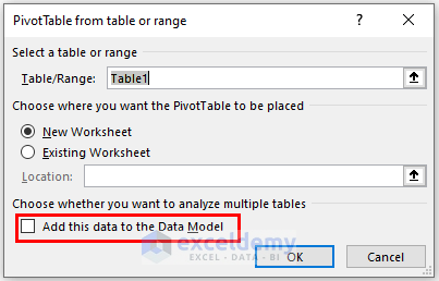
- In the PivotTable from table or range dialog box, you’ll see that the Table/Range box is already filled (based on your selection).
- Choose where you want to place the pivot table (e.g., New Worksheet) and click OK.
- You’ll have a blank pivot table in a new sheet.
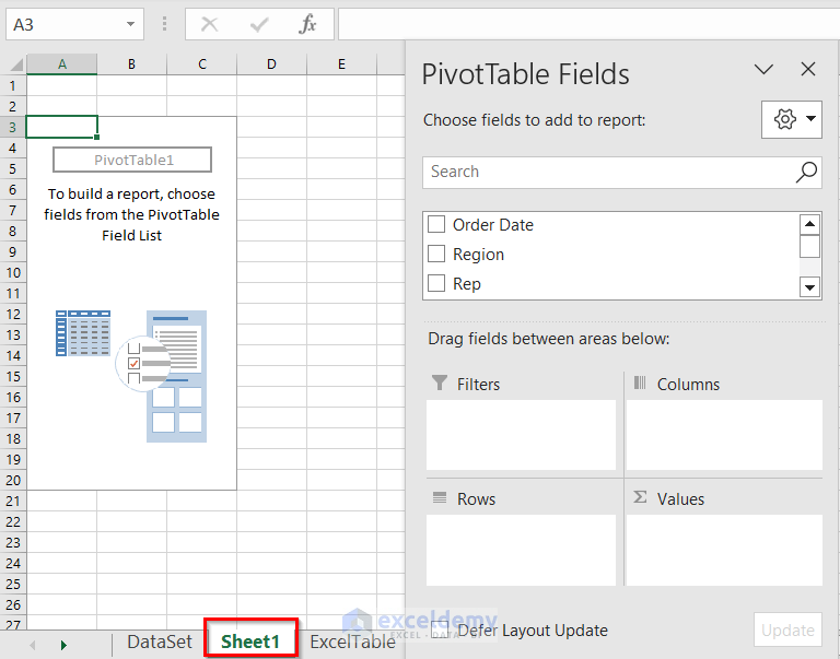
Example 1 – Defining a New Group with Specific Text Items
Step 1 – Prepare the Pivot Table
-
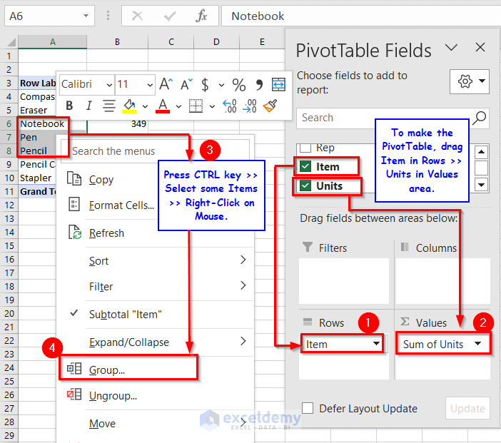
- Drag the relevant fields into their respective areas within the blank pivot table.
- Drag the “Item” field to the “Rows” area and the “Units” field to the “Values” area. The “Units” will be displayed as the sum of units.
Step 2 – Creating a Custom Group
-
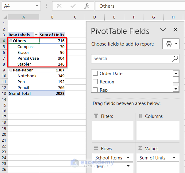
- In this section, we’ll create a group containing specific text items (in this case, “Notebook,” “Pen,” and “Pencil”).
- Follow these steps:
- Press the CTRL key.
- Select the desired items (Notebook, Pen, and Pencil).
- Right-click your mouse and choose Group from the context menu.
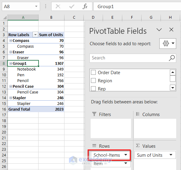
- You’ll see a new group named “Group1” containing the selected items. Note that in the “Rows” area, these items are labeled as “Item2.”

Step 3 – Renaming the Group
-
- Let’s change the default name of Group1:
- Select Group1.
- A new tab called PivotTable Analyze will appear.
- Go to PivotTable Analyze and choose Field Settings from the active field.
- Let’s change the default name of Group1:
-
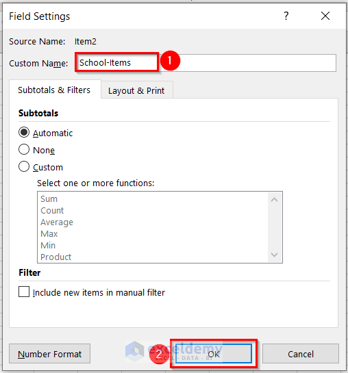
- In the “Field Settings” dialog box:
- Enter a custom name (e.g., “School-Items”) in the Custom Name box.
- In the “Field Settings” dialog box:
- Press OK.
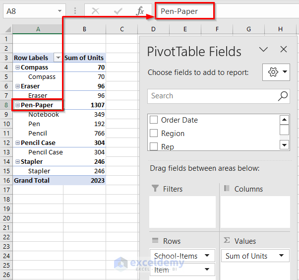
- The field previously known as Group1 will display as School-Items. To change the name further, use the Formula Bar.
- Additional Groups
- You can create other groups with different items and assign appropriate names by repeating the process.
Example 2 – Grouping Numbers in a Pivot Table
Step 1 – Prepare the Pivot Table
-
- Drag the Region field to the Rows area.
- Drag the Total Sales field to both the Rows and Values areas.

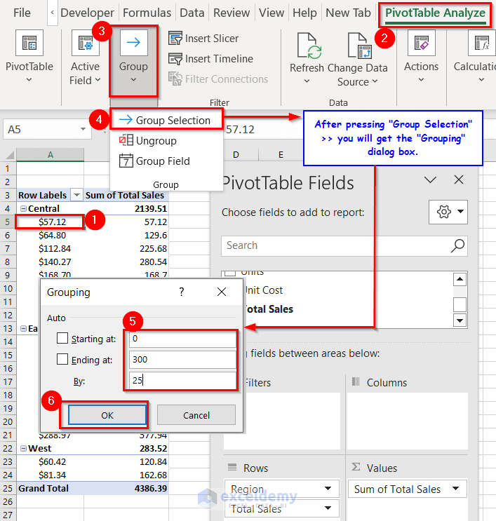
Step 2 – Grouping the Numbers
-
- Click on cell A5 within the pivot table.
- Go to the PivotTable Analyze tab.
- Click on Group and select Group Selection.
- In the Grouping dialog box:
- Specify the starting value (e.g., 0).
- Define the ending value (e.g., 300).
- Set the interval (e.g., 25).
- Press OK.

Step 3 – Understanding the Group
-
- The group will now be displayed in the pivot table.
- To determine how many sales fall within each range:
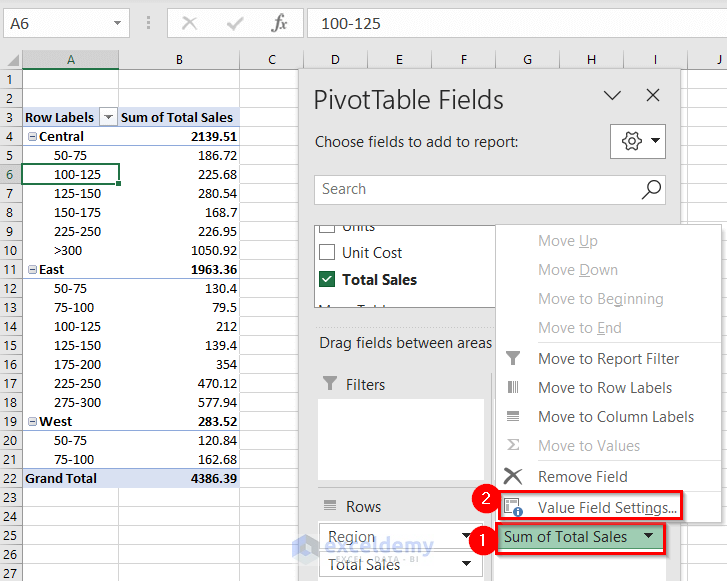
- Click the drop-down arrow next to Sum of Total Sales.
- Choose Value Field Settings.
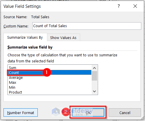
- In the Value Field Settings dialog box:
- Select Count from the Summarize value field by menu.
- Press OK.
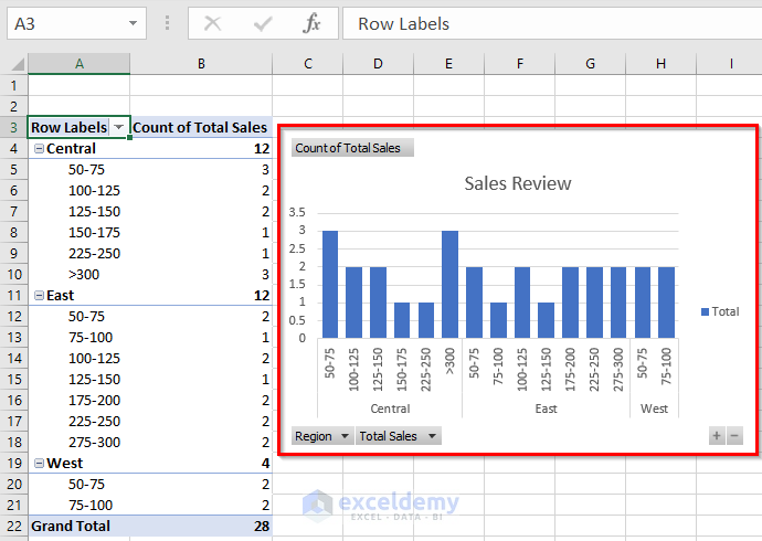
Step 4 – View the Results
-
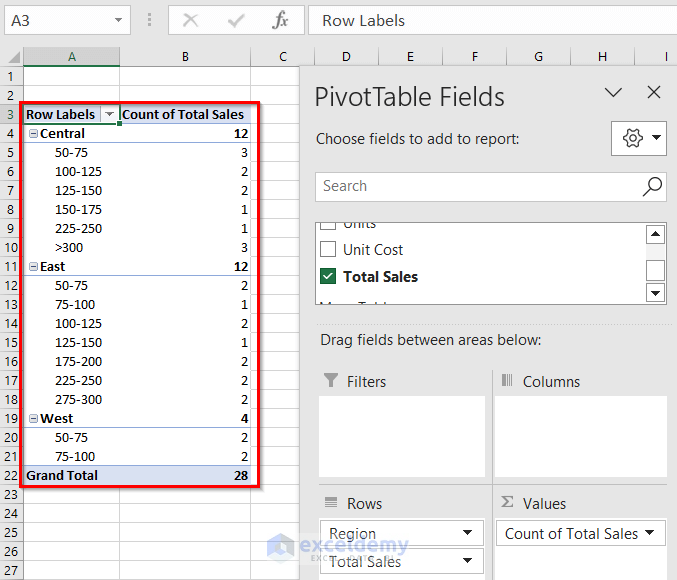
- You’ll now see the count of sales within each sales range.
Creating a Visual Representation of Grouped Numbers Using the PivotChart Option
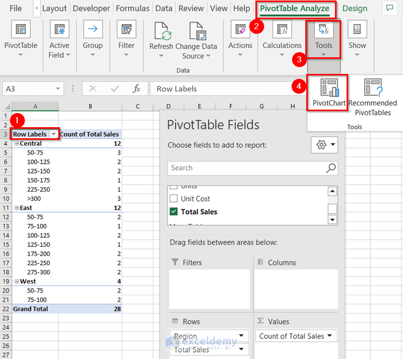
Step 1 – Activate the PivotChart
-
- Click on any cell within your pivot table to activate the PivotTable Analyze tab.
- From the PivotTable Analyze tab, go to the Tools option and select PivotChart.
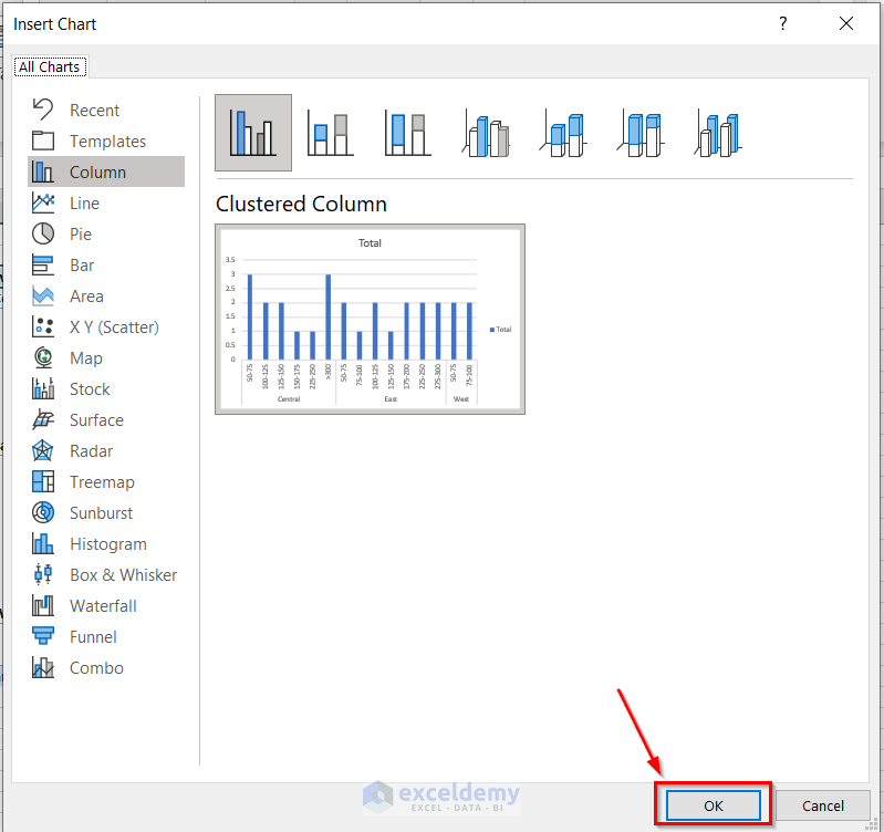
Step 2 – Insert Chart
-
- The Insert Chart dialog box will appear.
- The default selection will be the Clustered Column chart. Press OK.
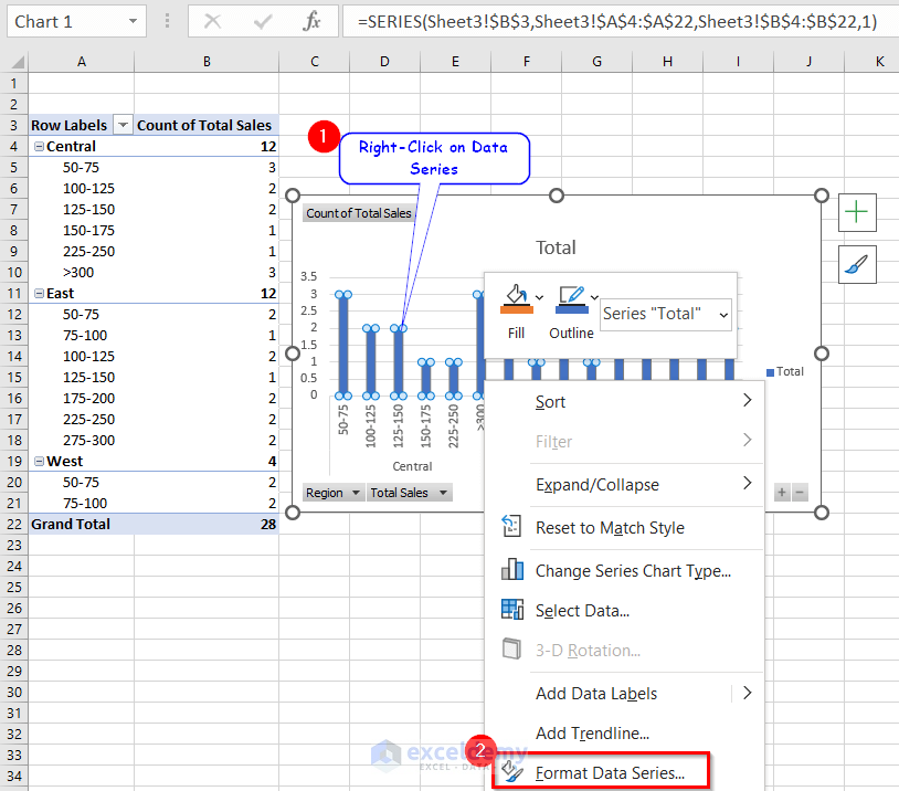
Step 3 – Format Data Series
-
- Right-click on the data series (the clustered column) within the chart.
- Choose Format Data Series from the context menu.
- The Format Data Series options will appear at the right-most corner of the Excel sheet.
Step 4 – Adjust Gap Width
-
- To improve the visual appearance:
- Decrease the gap width between columns.
- This adjustment can be made within the Format Data Series options.
- To improve the visual appearance:
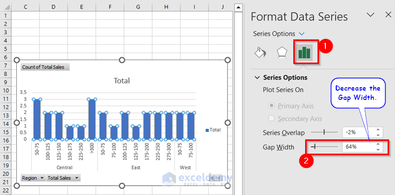
By following these steps, you’ll create a visual representation of your grouped data using a clustered column chart.
Example 3 – Grouping Dates with Pivot Table in Excel
Step 1 – Built-in Date Grouping
-
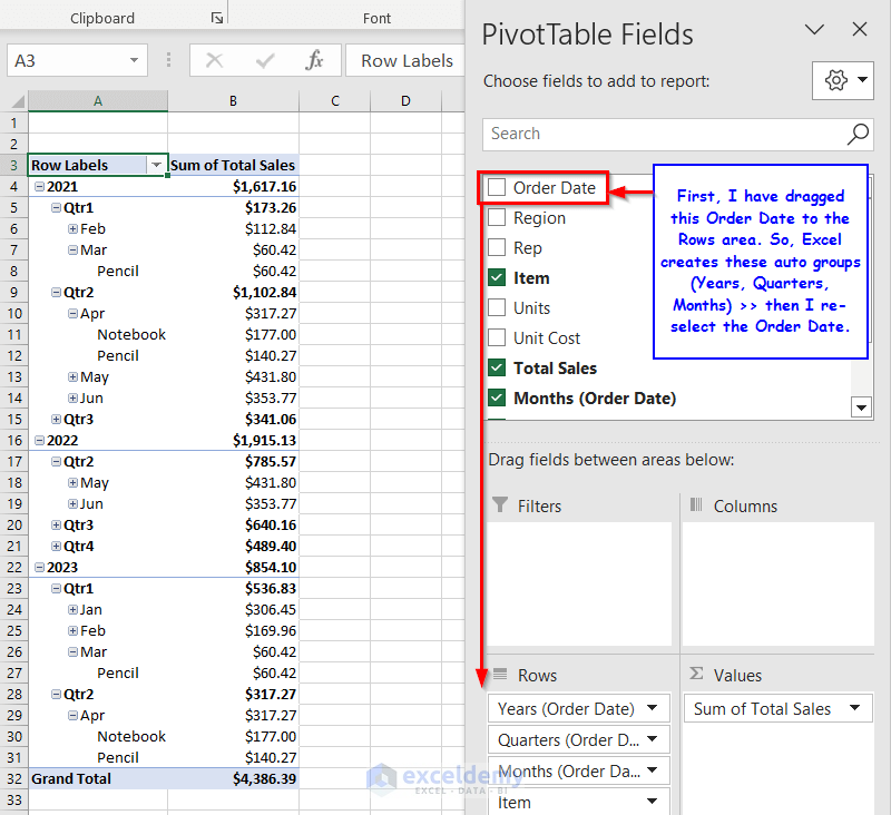
- The dataset includes a field named Order Date containing date values.
- Drag the Order Date field to the Rows area of your pivot table.
- Excel will automatically create date groups such as Years, Quarters, and Months.
- Initially, the date field is divided into years, then further into quarters, and finally into months.
- Under the Months group, individual dates are displayed. If you want to remove the exact date, simply drag the Order Date from the Rows area to the back.
Step 2 – Manual Date Grouping in Pivot Table
-
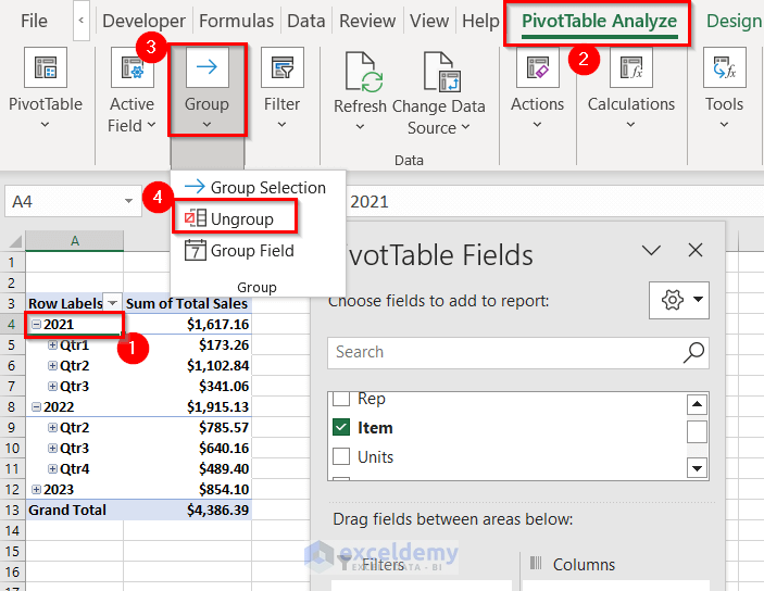
- To create a custom date group, first ungroup the auto-generated groups.
- Select any value from the grouped data.
- Go to the PivotTable Analyze tab and choose Ungroup from the Group menu.
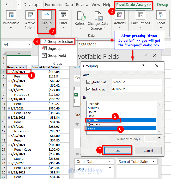
- Click on cell A4.
- From the PivotTable Analyze tab, select Group and then choose Group Selection.
- The Grouping dialog box will appear.
- Define the date range by specifying the Starting at (e.g., 2/26/2021) and Ending at (e.g., 4/19/2023) values.
- Select your preferred grouping options and click OK.
-
- As a result, you’ll have a custom group of years and months. If you’ve kept the Item field in the Rows area, the items will align with the custom group.

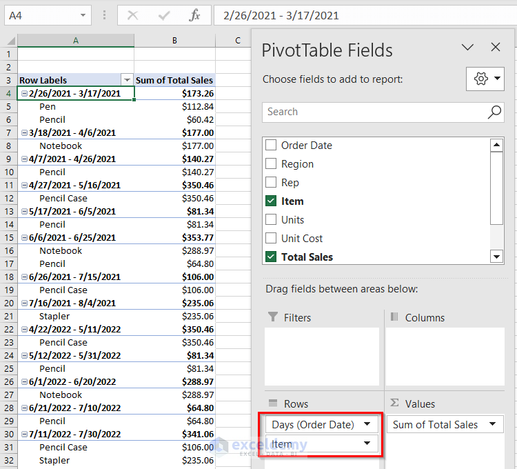
Step 3 – Use a Specific Range to Group Date Data in a Pivot Table
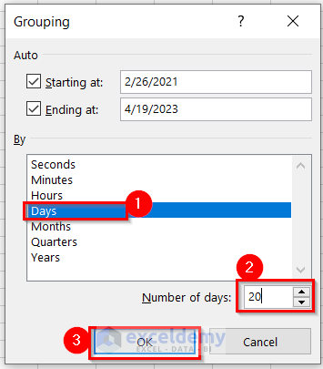
- Select Days for Grouping:
- Open the Grouping dialog box (similar to the previous example).
- Under the By options, choose Days.
- Specify the number of days as the class interval for your custom group.
- Click OK.
- Note: To create a defined class interval for date values, ensure that only the Days option is selected. Uncheck other options if they are selected.
Step 4 – Creating Custom Date Groups
-
- Once you’ve set the class interval, Excel will create custom date groups based on the specified range.
- You can also create groups with a class interval of one week (7 days) by adjusting the Number of days value accordingly.
- For example, if you want to see the group for a 4-week period, set the “Number of days” to 28 (4 weeks × 7 days = 28 days).
How to Disable Automatic Grouping in an Excel Pivot Table
If you prefer not to have Excel automatically group date values in your pivot table, follow these steps:
- Disable Automatic Grouping
- Go to the top ribbon of your Excel sheet.
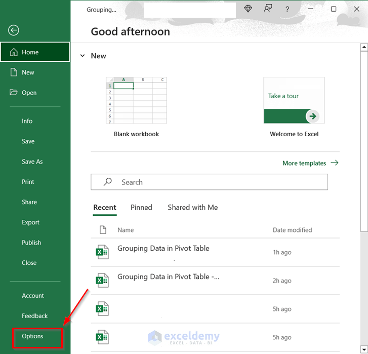
- Click on the File tab.
- In the resulting window, select Options.
-
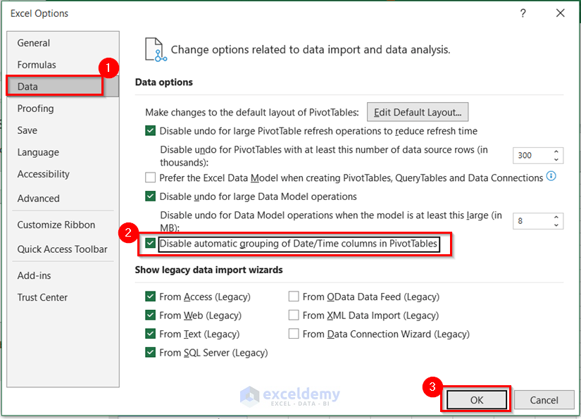
- The Excel Options dialog box will appear.
- Navigate to the Data section.
- Check the box labeled Disable automatic grouping of Date/Time columns in PivotTables.
- Press OK.
- Now, when you drag any field with date values, automatic grouping will be disabled.
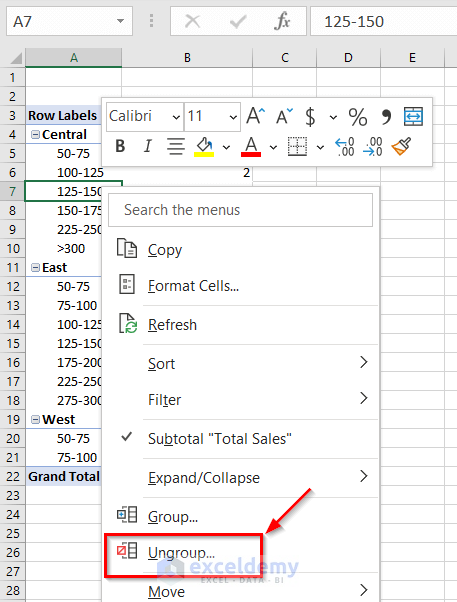
How to Ungroup Data in an Excel Pivot Table
- Alternative Ungrouping Method
- Right-click on any grouped cell within the pivot table.
- From the context menu, select Ungroup.
- All the grouped data will be ungrouped.
That’s it! You now know how to create custom date groups, disable automatic grouping, and ungroup data in Excel pivot tables.
Common Problems with Grouping in an Excel Pivot Table
- Data Model Option: When inserting a pivot table, if you check the option Add this data to the Data Model, you won’t be able to group any text or number data in that pivot table. In this case, grouping is only possible for fields with date values. To avoid this limitation, refrain from selecting the Add this data to the Data Model option.
- Blank Cells: Ensure that your dataset doesn’t contain any blank cells. Having blank cells will create an additional group named “blank,” which might cause inconvenience.
- Mixing Text and Numbers: When creating a group based on numbers, avoid mixing text values with numeric data. If your dataset includes both text and numeric values, you won’t be able to create a group based solely on numbers.
- Linked Pivot Tables: Be aware that pivot tables created from the same dataset are linked to each other. If you create a group in one pivot table, it affects all other pivot tables using the same data. To prevent this, follow the steps below:
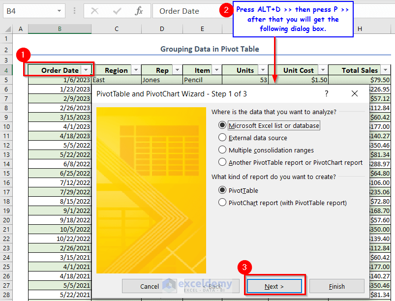
- Press ALT+D, then press P to open the “PivotTable and PivotChart Wizard – Step 1 of 3” dialog box.
- Click Next in that dialog box.
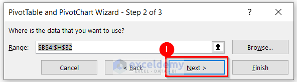
- In the “PivotTable and PivotChart Wizard – Step 2 of 3,” click Next again.
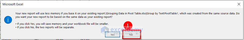
- When prompted with information from Microsoft Excel, choose No.
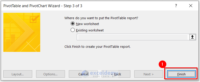
- In the final dialog box (“PivotTable and PivotChart Wizard – Step 3 of 3”), press Finish.
- You’ll now have a blank pivot table. Drag fields into it and create your preferred groups.
Preventing Pivot Table Grouping Across Multiple Pivot Tables in Excel
When multiple pivot tables share the same source data, grouping in one pivot table can impact other pivot tables. To avoid this issue, follow these steps to create pivot tables in a way that prevents grouping from affecting others:
- Press ALT+D, then press P to open the “PivotTable and PivotChart Wizard – Step 1 of 3” dialog box.
- Click Next in that dialog box.
- In the “PivotTable and PivotChart Wizard – Step 2 of 3,” click Next again.
- When prompted with information from Microsoft Excel, choose No.
- In the final dialog box (“PivotTable and PivotChart Wizard – Step 3 of 3”), press Finish.
- You’ll now have a blank pivot table. Drag fields into it and create your preferred groups.
Filtering Data in an Excel Pivot Table
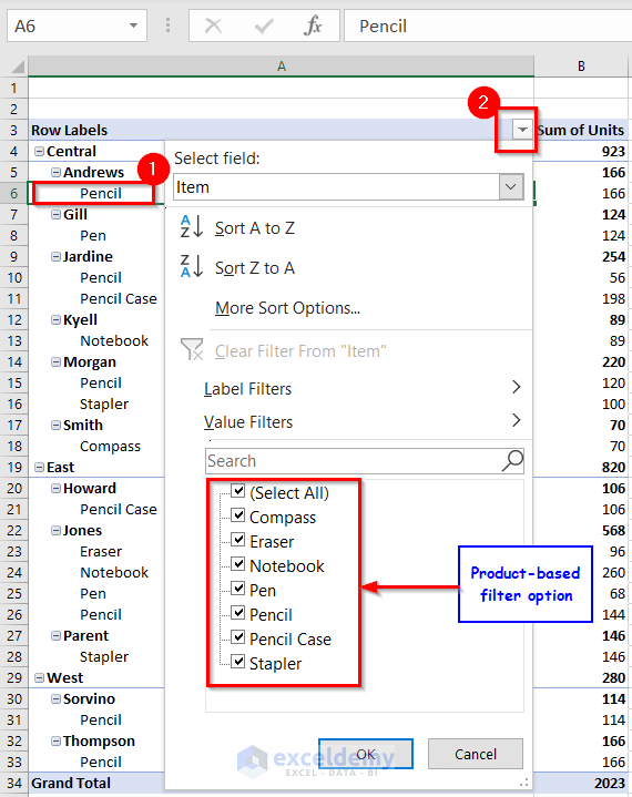
Before filtering, decide which value you want to filter the data based on. Follow these steps:
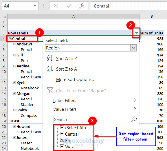
- If you select any cell containing a region, click the drop-down arrow beside Row Labels to access the region-based filter option.
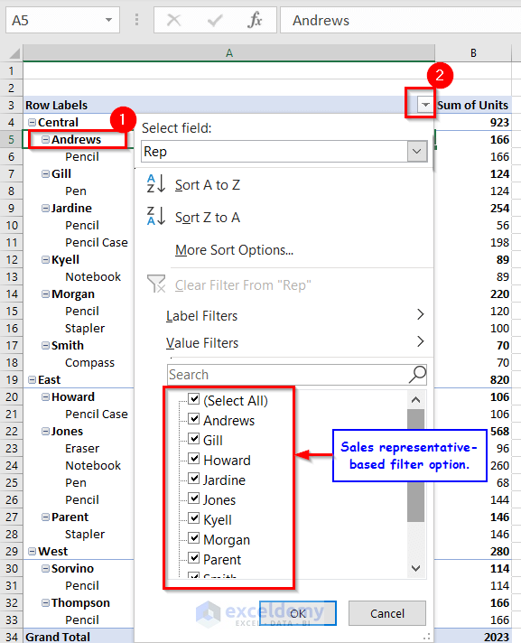
- Similarly, if you select any cell with the name of a representative, use the drop-down arrow beside Row Labels for the representative-based filter option.
- For item-based filtering, select any cell containing an item, and then use the drop-down arrow beside Row Labels.
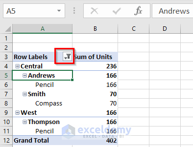
We have filtered the data based on the sales representative.
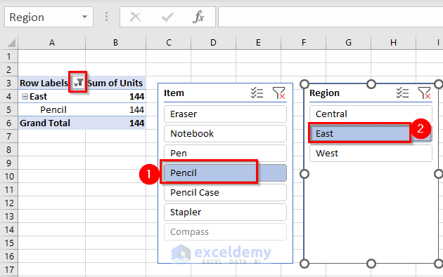
Adding a Slicer to an Excel Pivot Table
Slicers provide another way to filter data in a pivot table. They display unique values of a field, allowing you to easily select specific values. To add a slicer:
- Click any cell within the pivot table.
- Go to the PivotTable Analyze tab.
- Under Filter, click Insert Slicer.
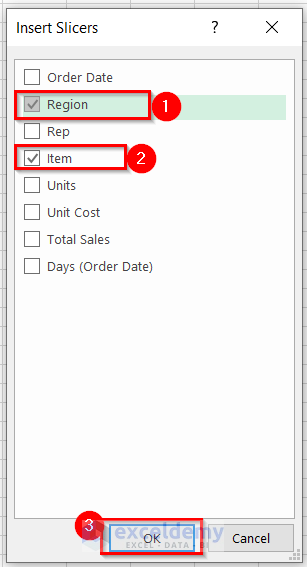
- Choose the field you want to use as a slicer.
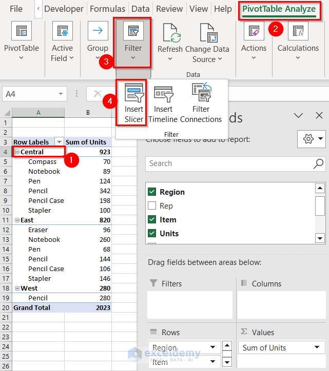
- Now you can filter your pivot table using the slicer values.
Frequently Asked Questions
Can I Sort Values in a Pivot Table?
Yes, you can sort values in a pivot table. To do so:
- Click the drop-down arrow beside the Row Labels.
- You’ll find options to sort the data based on your preferences.
Where Are PivotTable Tools?
When you activate any cell within the pivot table, two contextual tabs appear: PivotTable Analyze and Design. These tabs contain various tools for working with pivot tables.
Download the Practice Workbook
You can download the practice workbook from here:

