Excel Slicer Multiple Columns: 3 Examples

Method 1 – Excel Slicer with Multiple Columns

Find all the columns in the Excel slicer in a single column. You can see the below image.

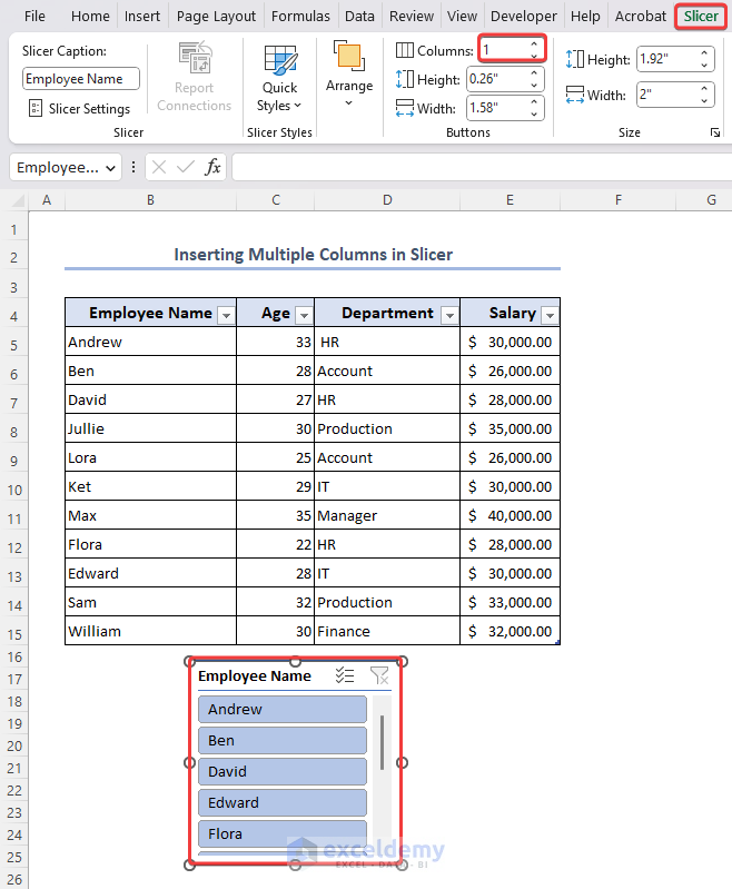
Sometimes there is so much data in a column that you can face trouble to filter your desired values. You can distribute data in multiple columns in a slicer. To do so,

• We already know how to add a slicer in Excel. Click on the slicer which you want to divide into multiple columns.
• Go to the Slicer menu bar.
• Select the Column bar and enter the number of columns you want to divide the slicer.
• Use the upper and lower cursor of the Column number bar to customize the column number.
• In the column number bar, we enter 3, so you will find the slicer divide into three columns.

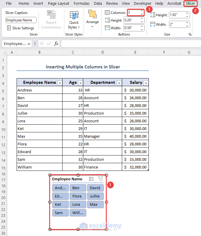
We can see there are three columns in the slicer.

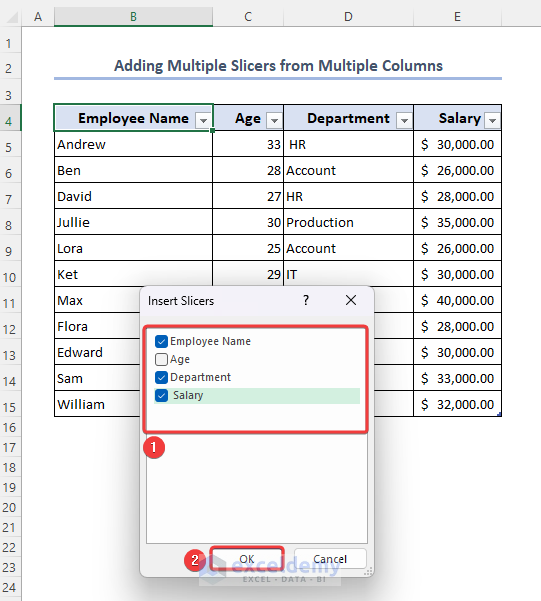
Method 2 – Add Multiple Slicers for Multiple Columns in Excel

• Go to Insert the Slicer dialog box; find all the column headers.
• Check the headers you want to add as a slice and click OK.

• Multiple slicers will be added to your worksheet.

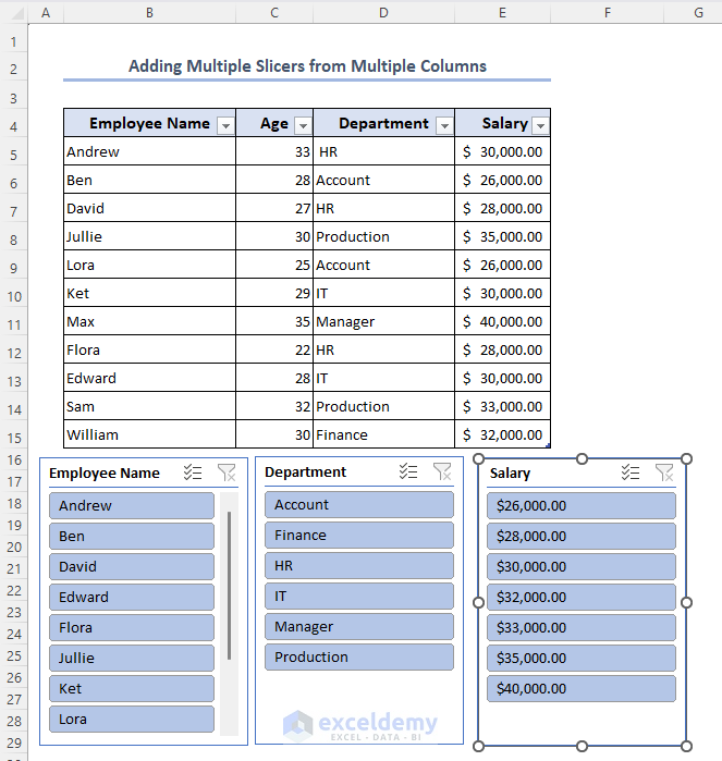
You will be able to filter data by selecting options from different slicers.

Method 3 – Select Multiple Items in a Single Slicer

• Select the marked symbol (Multi-Select) and click on the items that you want to filter.
• Find the selected items filtered in your table.

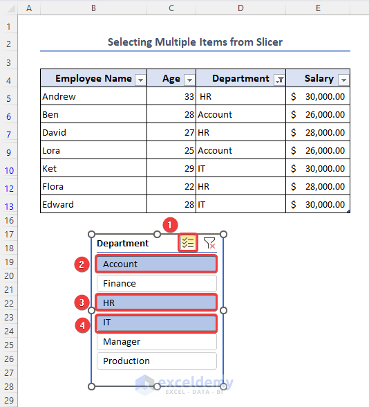
Use the Ctrl key to select multiple items from the slicer.

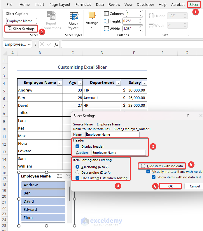
How to Customize Excel Slicer

• Go to the Slicer menu and select the Slicer Settings
• Find a box where you can change the Slicer Name and item arrangement and check to hide items with no data.
• Click on OK to apply all the settings.

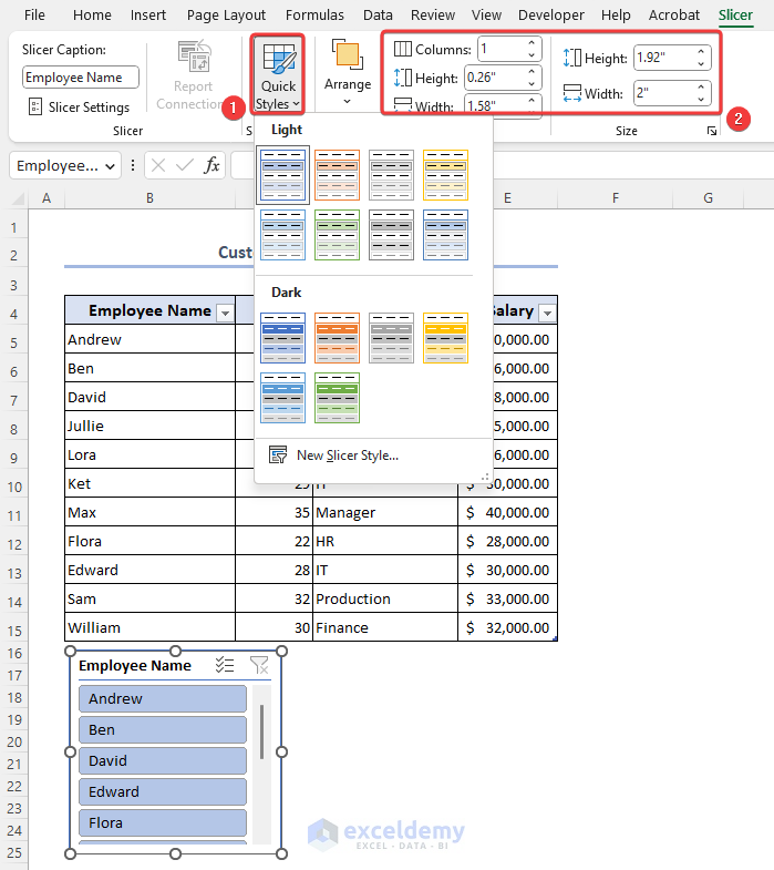
• Change the slicer style by expanding to the Quick Styles
• Change the slicer column height and width.

Benefits of Using Multiple Column Slicer

Slicers have so many advantages to use on a dataset. Moreover, a multiple-column slicer has some more benefits as well. They are-

• Multiple-column slicers provide a holistic view of your data, allowing you to analyze multiple dimensions simultaneously. Slice and dice your data based on various criteria, facilitating deeper insights and a better understanding of complex relationships.
• You can create more comprehensive and interactive visualizations using slicers with multiple columns. Easily switch between different combinations of columns, enabling you to present your data in a visually appealing and informative manner.
• With multiple-column slicers, you can streamline your data filtering process. Instead of applying individual filters to each column separately, make selections across multiple columns, saving time and effort.
• Sharing workbooks with multiple-column slicers simplifies collaboration among team members. Explore the data using the slicers, ensuring consistent analysis and fostering effective decision-making.

Frequently Asked Questions

1. Can I customize the appearance and behavior of slicers for multiple columns?

Yes, Excel provides various customization options for slicers. You can change their size, color, and layout, and connect them to multiple pivot tables or charts. Additionally, you can control how slicers interact with each other and the data by adjusting options in the slicer settings.

2. Can I use slicers to filter data in regular Excel tables, not just pivot tables?

Yes, slicers can be used to filter data in regular Excel tables as well. Simply select the table range, go to the “Insert” tab, and create slicers using the same steps mentioned earlier.

3. Can I remove slicers from my worksheet once I no longer need them?

Yes, you can remove slicers from your worksheet by selecting the slicer(s) and pressing the “Delete” key. Alternatively, you can right-click on a slicer and choose the “Delete” option.

4. Can I save and reuse slicers in different Excel workbooks?

Unfortunately, Excel doesn’t provide a direct option to save and reuse slicers across different workbooks. However, you can copy and paste slicers between workbooks manually or use VBA programming to automate the process.

5. Are there any limitations or considerations when using slicers for multiple columns in Excel?

One important consideration is that slicers filter data in an “OR” logic. It means that selecting values in different slicers will display any data that matches all the selected values. Additionally, the number of slicers you can add to a worksheet may be limited based on the available screen space.

Things to Remember

• Carefully insert the range while inserting a table.
• Add slicers as per your requirement.
• Input multiple columns in a slicer for better visualization of many items.
• Check the slicer header according to your requirements.
• You can use this process to apply the slicer in Pivot Table

Download Practice Workbook

You can find the practice sheet here.