Dataset Overview:
-
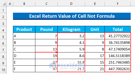
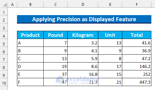
- We have a dataset with 5 columns: Product, Pound, Kilogram, Unit, and Total.
- The data is given in pounds, and we want to convert it to kilograms.
- Our goal is to calculate the total product weights based on the display value in column D.
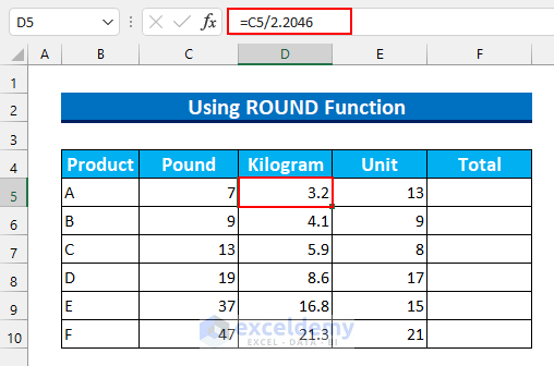
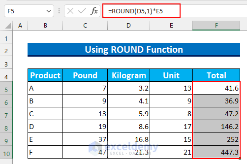
Method 1 – Using ROUND Function
1 kilogram = 2.2046 pounds, therefore 7 pounds (Cell C5) = 3.17 kilograms and rounded = 3.2 kilograms (Cell D5).
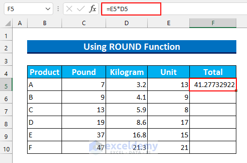
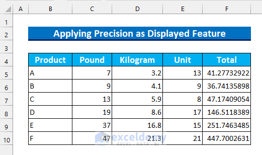
If we multiply the weight (3.2kg) by the number of units (13 in cell E5), then we will get a different output from our intention. We expect the result to be 41.6, however, we will get 41.27732922 as the result.
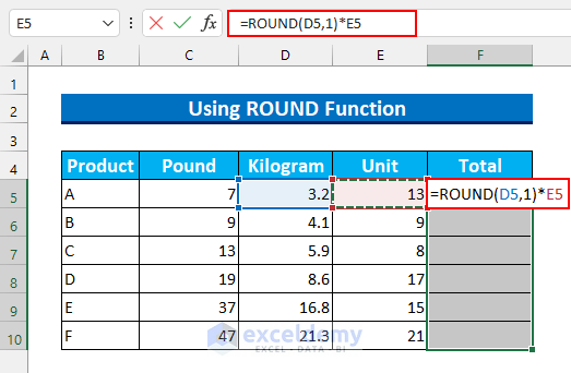
Steps:
- First, select the cell range F5:F10.
- Enter the following formula:
=ROUND(D5,1)*E5
Formula Breakdown
-
- The ROUND function rounds the value from cell D5 to one decimal place.
- So, 7 divided by 2.2046 will be 3.2.
- We multiplied it by the number of units sold.
- We will get our desired result of 41.6.
- Press CTRL+ENTER to autofill the formula for the remaining cells.
This ensures that Excel uses the display value rather than the full formula for calculations.
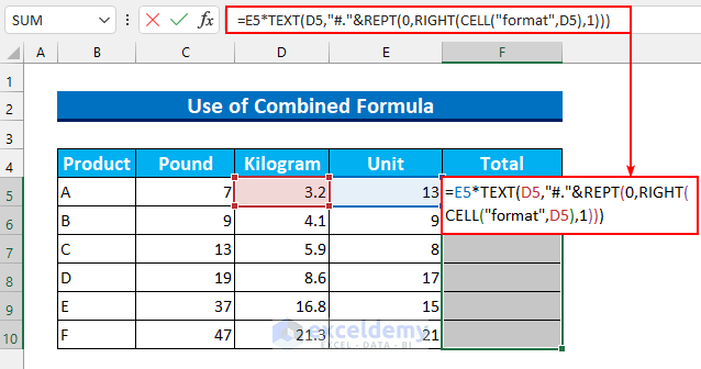
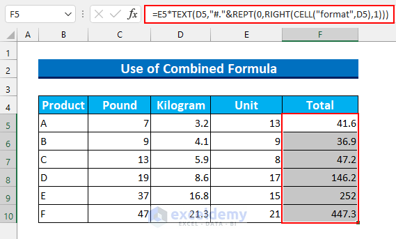
Method 2 – Combined Formula Approach
Steps:
- Select the cell range F5:F10.
- Enter the following formula:
=E5*TEXT(D5,"#."&REPT(0,RIGHT(CELL("format",D5),1)))
Formula Breakdown
-
- The main part of the formula is the TEXT function, which preserves the cell contents as they appear.
- The RIGHT function extracts the number of decimal places from the format of cell D5.
- For example, if D5 displays numbers with one decimal place (e.g., “F1”), the result will be 41.6.
- The REPT function repeats the value 0 exactly once.
- Multiply this adjusted value by the units (cell E5) to get the desired output.
- Press CTRL+ENTER to autofill the formula for the remaining cells.
This method ensures that Excel calculates based on the display value, not the full formula.
Method 3 – Set Precision as Displayed
Objective:
- Our goal is to ensure that Excel uses the displayed value (as seen by the user) for calculations, rather than the full formula.
Steps:
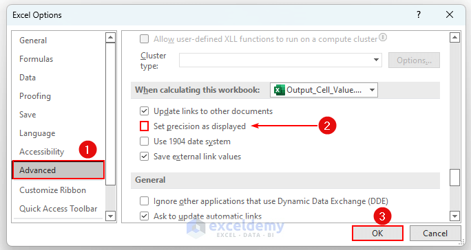
- Press ALT, then F, and finally T to open the Excel Options window.
- Navigate to the Advanced tab.
- Under the When calculating this workbook section, select Set precision as displayed.
- Click OK.
- A warning message will appear; confirm by clicking OK.
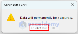
- Once enabled, Excel will automatically adjust the values based on their displayed precision.
In summary, this method allows you to return the value of a cell without using the underlying formula. By setting precision as displayed, you ensure that calculations consider the rounded display value rather than the full formula.
Read More: Convert Formula to Value in Multiple Cells in Excel
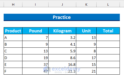
Practice Section
We have added a practice dataset for each method in the Excel file.to allow you to follow along.
Download Practice Workbook
You can download the practice workbook from here:
Related Articles
- How to Stop Formula to Convert into Value Automatically in Excel
- How to Convert Formula to Value Automatically in Excel
- How to Convert Formula Result to Text String in Excel
- Excel VBA: Convert Formula to Value Automatically
- Putting Result of a Formula in Another Cell in Excel
<< Go Back to Convert Formula to Value in Excel | Excel Formulas | Learn Excel
Get FREE Advanced Excel Exercises with Solutions!

Hello Rafiul,
Got a problem with the IF function not returning a time value hh:mm but either returning the formula or the cell number where I tried to use a workaround.
Problem:
1. Lock off 23:15
2. Lock on 04:15
3. Lock off 05:05
4. Lock 0n 07:00
Total time is the difference between 1. and 4. but if 3. and 4. did not take place the Total time is between 1. and 2.
=IF(MOD(B43-B30,1))>(MOD(B35-B30,1)),“MOD(B43-B30,1)”,“MOD(B35-B30,1)”)
Dear Peter Summers
Thanks for visiting our blog and sharing your problem. You wanted to return a time value with “hh:mm”. To do so, you have to enhance your formula with the help of the TEXT function:
Hopefully, you have found the idea helpful; good luck.
Regards
Lutfor Rahman Shimanto
ExcelDemy