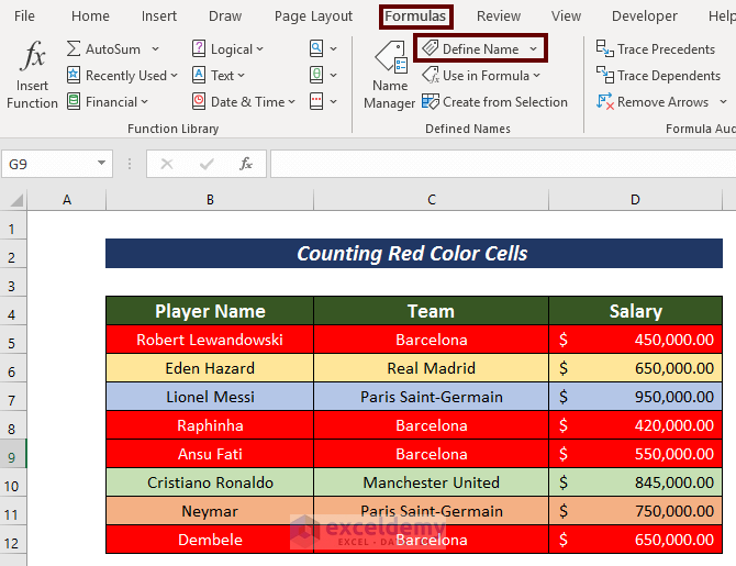
Method 1 – Counting Red Color Cells
- Define Name
- Applying the COUNTIFS Function
Steps:
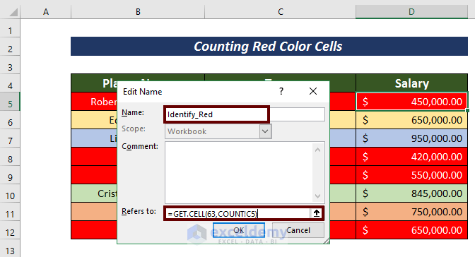
An Edit Name wizard will appear.
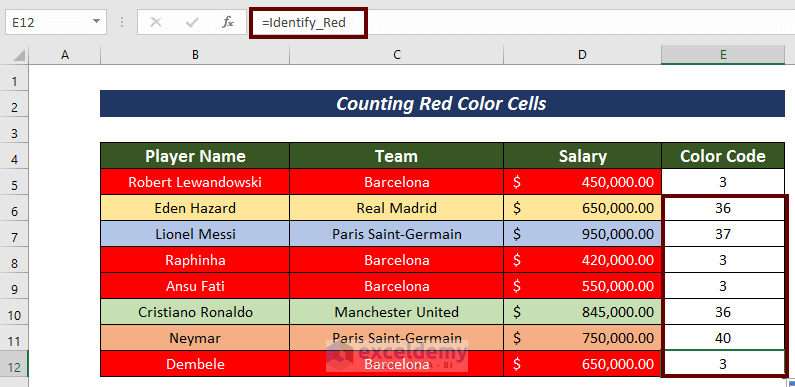
- Set a name in the Name section (i.e. Identify_Red).
- Input the following formula in the Refers to section.
=GET.CELL(63,COUNT!B15)63 returns the fill (background) color of the cell. COUNT! refers to the sheet name. $B15 is the cell address of the first cell to consider in Column B.
- Press OK.
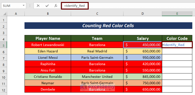
- Create a new column (i.e. Color Code) to have the code number of the color.
- Apply the following formula in the E5 cell of the Color Code.
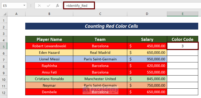
=Identify_RedWe mentioned the defined name.
- Press ENTER to have the color code.
- Use Fill Handle to AutoFill the rest columns.
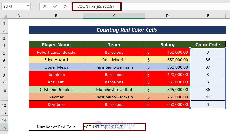
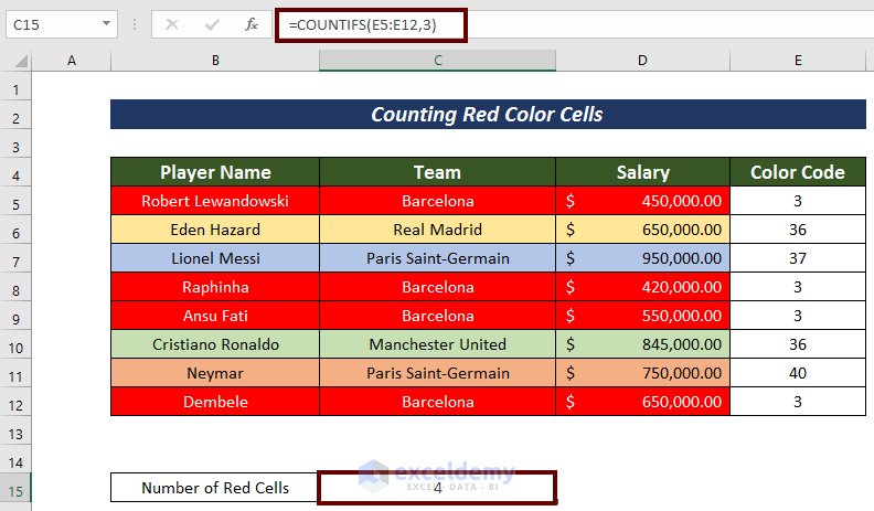
- Input the following formula to have the Number of Red Cells.
=COUNTIFS(E5:E12,3)The COUNTIFS function counts the red cells in cells E5:E12 as the red color code is 3.
- Press ENTER to have the output.
We can simply count the cells if the red color has been applied.
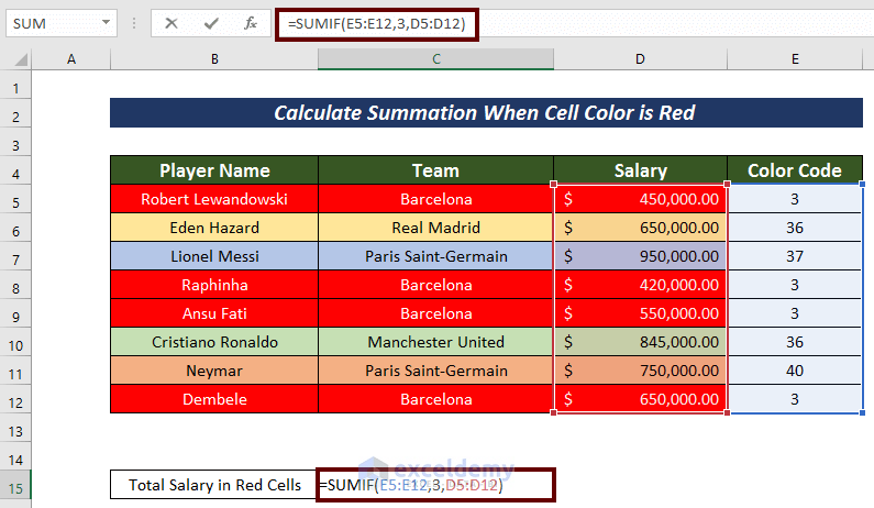
Method 2 – Calculate Summation When Cell Color Is Red
Steps:
- Find the Color Code using the same method mentioned in the previous section.
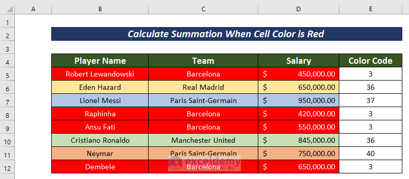
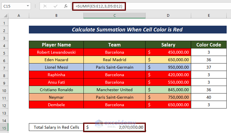
- Apply the formula mentioned below to have the summation of the salary in red cells.
=SUMIF(E5:E12,3,D5:D12)The SUMIF function looks through the range E5 to E12 whether any value matches with 3 or not. If they get matched, the connected values in the range D5:D12 are added.
- Press ENTER to have the Total Salary in Red Cells.
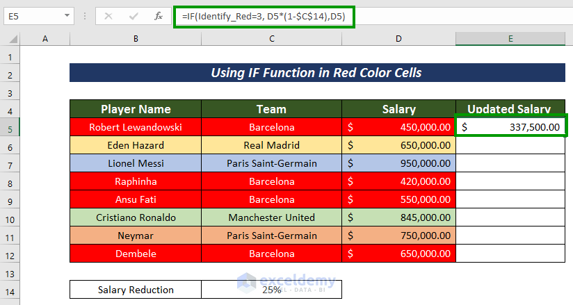
Method 3 – Using IF Function for Red Color Cell
The IF function can also be used in the red-colored cells to apply any specific function. We considered a 25% salary reduction for the salary connected with red-colored cells.
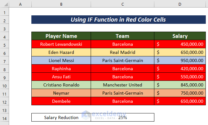
Steps:
- Ceate a new column to have the updated salary considering the salary reduction for red cells.
- Apply the following formula in the Updated Salary column.
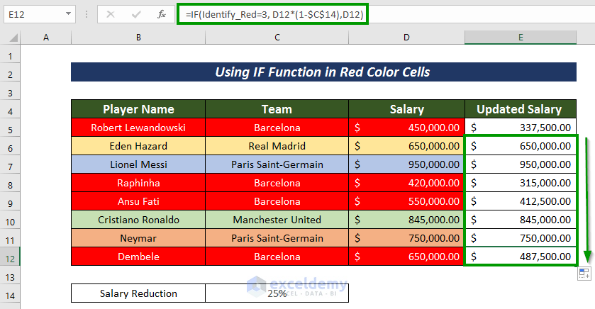
=IF(Identify_Red=3, D5*(1-$C$14),D5)We mentioned Identify_Red as a Define Name. The IF function checks whether the defined name matches the red color code. The salary reduction is applied, and the salary is updated.
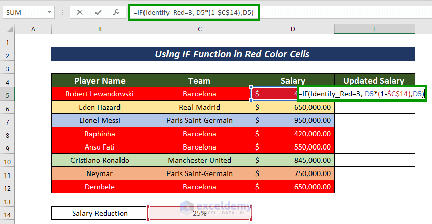
- Press ENTER to have the updated salary.
- Autofill the rest cells.
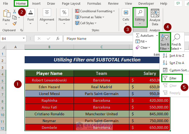
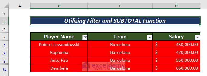
Method 4 – Utilizing Filter and SUBTOTAL Function on Cells of Red Color
Steps:
- Select the entire dataset.
- Go to the Home tab.
- Select Editing from the ribbon and choose Sort & Filter.
- Pick the Filter option.
- Click on the button in the title section.
- Choose the red color from the Filter by Color option.
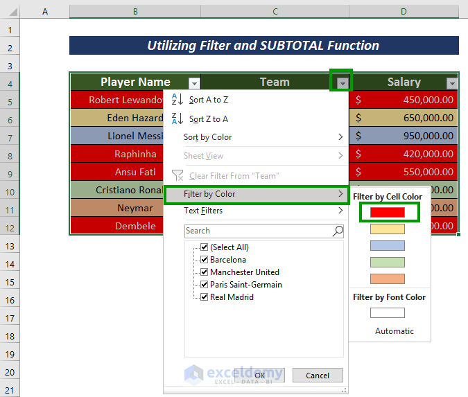
This is how we can filter the red cells.
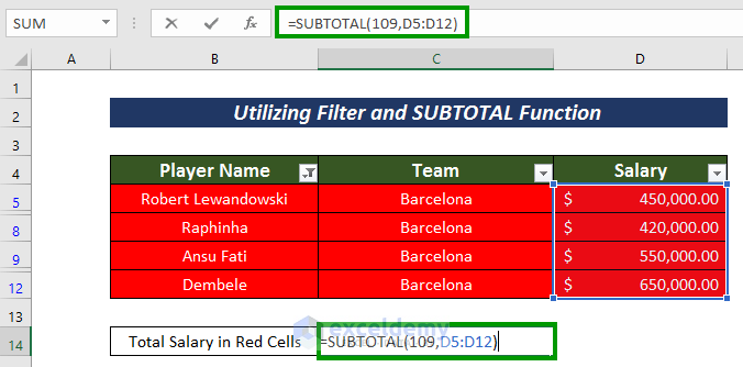
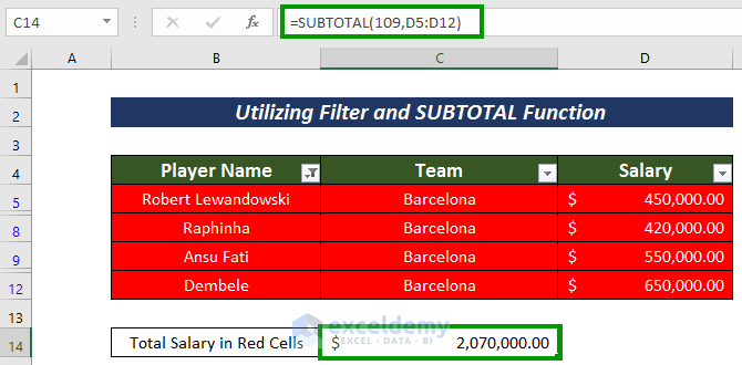
- Apply the following formula to have the Total Salary in Red Cells.
=SUBTOTAL(109,D5:D12)The SUBTOTAL function considers the sum operation for the visible rows within D5:D12 cells by 109 numbers.
- Hit ENTER to have our desired result.
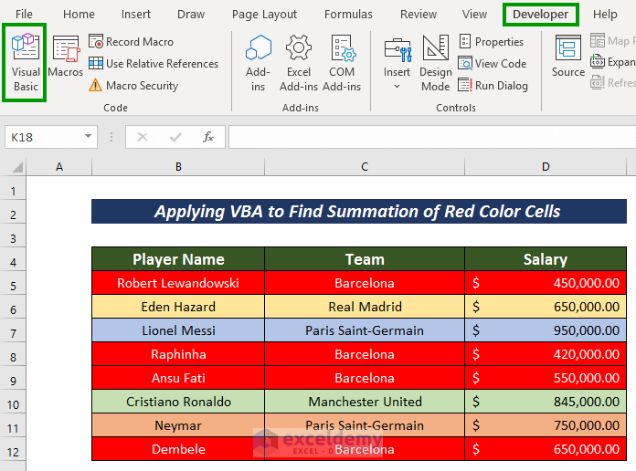
Method 5 – Applying VBA to Find Summation of Red Color Cells
Steps:
- Go to the Developer tab first.
- Click on Visual Basic from the ribbon.
Press ALT + F11 to perform the same thing.
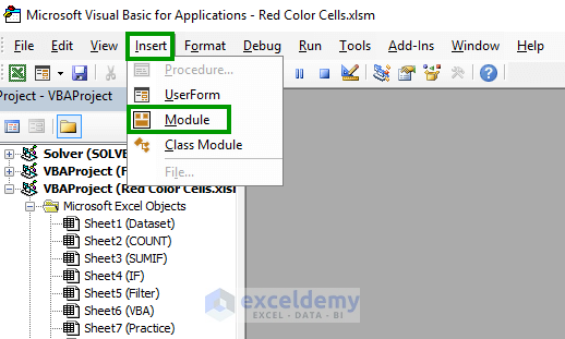
- Select the Insert tab.
- Click Module.
- Write the following Code.
Function Red_Cells_Summation (p As Range, q As Range)
Dim m As Long
Dim n As Integer
n = p.Interior.ColorIndex
For Each i In q
If i.Interior.ColorIndex = n Then
m = WorksheetFunction.Sum(i, m)
End If
Next i
Red_Cells_Summation = m
End Function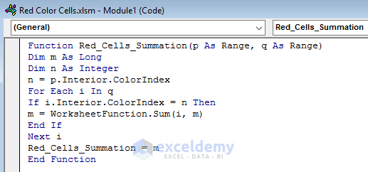
We considered Red_Cells_Summation as Sub_procedure. I also used the ColorIndex property to consider the cell color and WorksheetFunction.Sum to have the summation value.
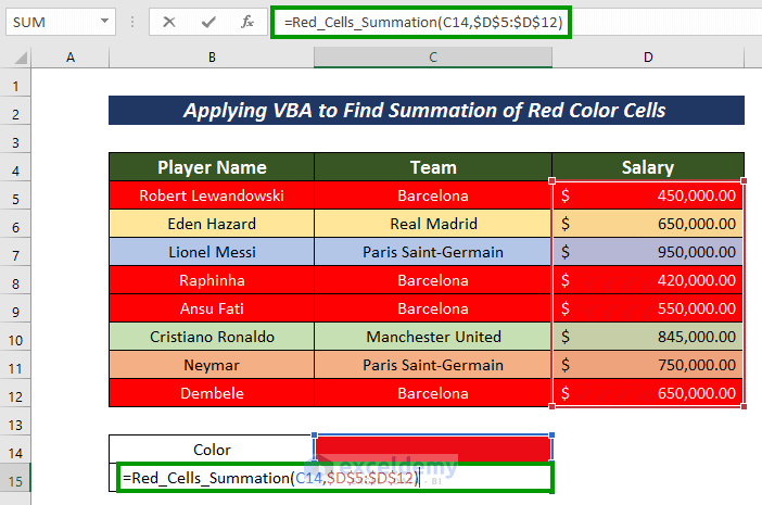
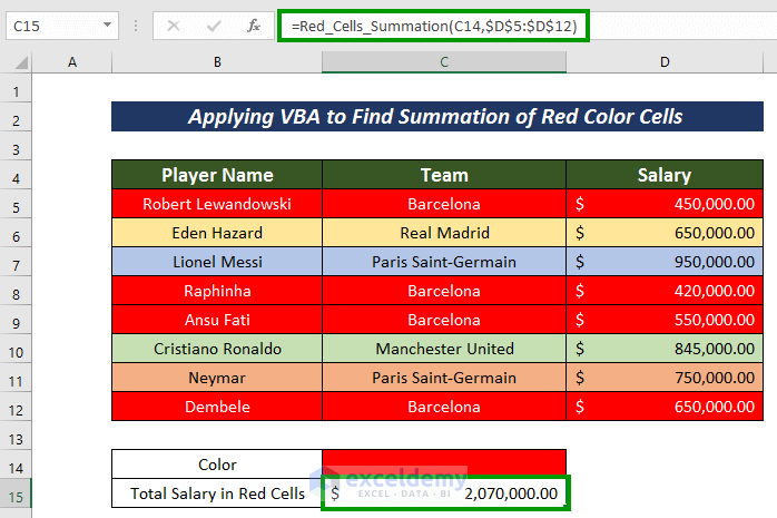
- Create the Color and Total Salary in Red Cells section on the worksheet.
- Input Red color in the Color section.
- Apply the following formula.
=Red_Cells_Summation(C14,$D$5:$D$12)Here, Red_Cells_Summation is a function that I mentioned in my VBA code. I have applied red color in cell C14 and applied the function in cell D5:D12.
- Press the ENTER button to have the summation value of red cells.
Download Practice Workbook
Related Articles
<< Go Back to Excel Get Cell Color | Excel Cell Format | Learn Excel
Get FREE Advanced Excel Exercises with Solutions!
