Dataset Overview
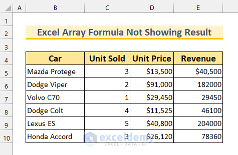
To illustrate our solutions, we’ll work with a dataset containing four columns: Car, Unit Sold, Unit Price, and Revenue. Our goal is to apply an array formula to determine the revenues for each type of car sold by a specific company.
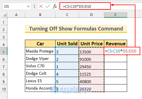
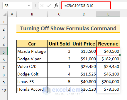
Solution 1 – Turning Off Show Formulas Command in Excel
- If the Show Formulas command is enabled, the sheet displays formulas instead of results.
- To address this:
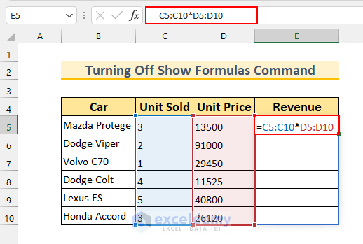
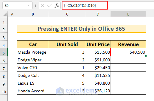
- In cell E5, enter the following formula:
=C5:C10*D5:D10
Formula Breakdown
- This array formula multiplies corresponding cells from columns C and D, yielding the value in column E.
- For instance, E5 = C5 * D5, E6 = C6 * D6, and so on.
- Press ENTER.
- Instead of showing the Excel array formula result, it will show us the array formula.
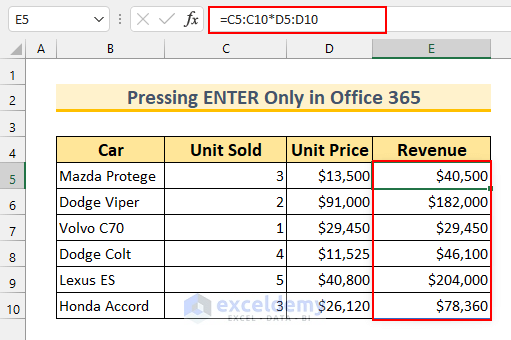
- If the array formula still shows as a formula, deselect Show Formulas from the Formulas tab.
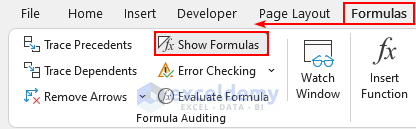
- The Excel array formula will show the result.
Solution 2 – Solving #SPILL! Error in Excel Array Formula to Show Result
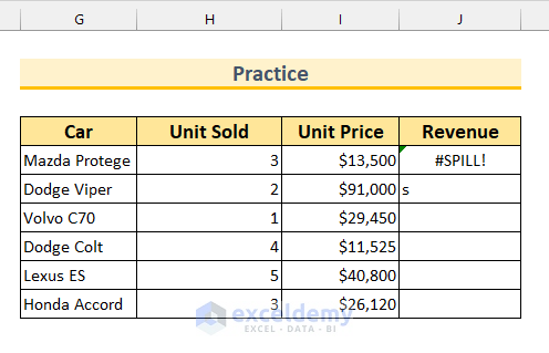
- In Excel 365, array formulas dynamically populate cells when you press ENTER.
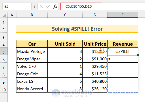
- If an existing value interferes, you’ll encounter the #SPILL error.
- To fix this:
- Enter the formula in cell E5:
=C5:C10*D5:D10
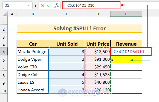
- Notice any existing value (e.g., “s”) in cell E6.
- Delete that value and press ENTER.
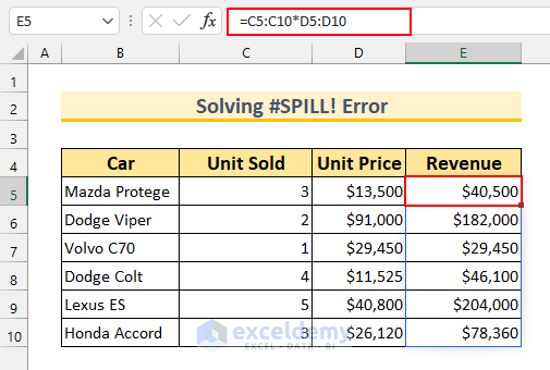
- So, our array formula will show the result.
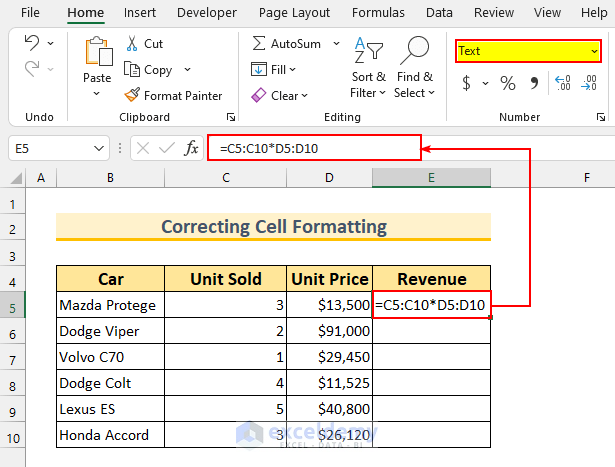
Solution 3 – Changing Cell Format to Fix Array Formula Display
- If a cell is formatted as Text, it shows the formula rather than the result.
- Rectify the Number Format:
- Enter the formula in cell E5:
=C5:C10*D5:D10
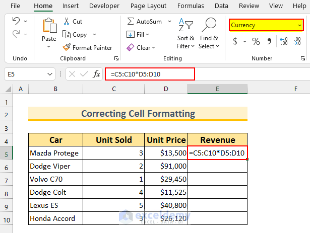
- Press ENTER.
- If the formula remains visible, change the cell format (e.g., select Currency format).
- Active the formula by double-clicking on cell E5.
- Press ENTER.
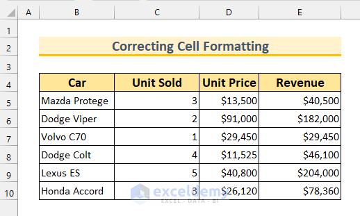
- The Excel array formula will return the desired output.
Read More: [Fixed!] Formula Not Working in Excel and Showing as Text
Solution 4 – Showing Result by Pressing Only ENTER in Excel Array Formula
- In Excel 365, use ENTER (not CTRL+SHIFT+ENTER) to calculate array formulas.
- To fix this:
- Enter the formula in cell E5:
=C5:C10*D5:D10
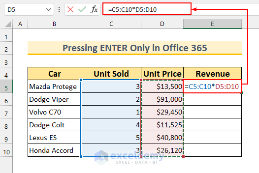
- Instead of CTRL+SHIFT+ENTER, press ENTER.
- Activate cell E5 by double-clicking on it.
- Press ENTER.
- The result will display as expected.
Read More: [Solved:] Excel Formula Not Working unless Double Click Cell
Things to Remember
- These solutions apply to Excel 365. For older versions (pre-Excel 2019), use CTRL+SHIFT+ENTER for array formulas (except for functions like AGGREGATE and SUMPRODUCT).
Practice Section
We have added a practice dataset for each method in the Excel file. You can follow along with our methods easily.
Download Practice Workbook
You can download the practice workbook from here:
Related Articles
- How to Refresh Formulas in Excel
- [Fixed!] SUM Formula Not Working in Excel
- [Fixed!]: Excel Formula Not Showing Correct Result
- Excel Formulas Not Calculating Automatically
- [Fixed!] Excel Formulas Not Working on Another Computer
- [Solved]: Excel Formulas Not Updating Until Save
<< Go Back To Formulas not Working in Excel | Excel Formulas | Learn Excel
Get FREE Advanced Excel Exercises with Solutions!

Hi. I was using the “mode.mult” function but for set of numbers with more than 1 mode, the function shows only 1 mode instead of 2 or more. I tried using the “ctrl+shift+enter” but it still only shows 1 mode. How do I fix this? Thank you.
Hello Cielo. Thank you for your question. I have tested the function on Excel 365, 2021, and 2013 versions. On first two version, you simply press ENTER and the formula will be spilled. However, in Excel 2013 if you press that, it will only show the first value.
Here, we have typed the formula in cell C5.
Then, pressed CTRL+SHIFT+ENTER. But, only the first value is seen.
To solve this, you need to follow these steps:
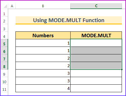
1. Select the cell ranges C5:C8 first.
2. Type the formula =MODE.MULT(B5:B11)
3. Press CTRL+SHIFT+ENTER. So, it will show all the mode values. Additionally, we have selected four cells, but there are only three outputs. Therefore, there is a “#N/A” for that reason.
Thank you for sharing your information.
Hello John,
You are most welcome. Thanks for your appreciation and feedback. Glad to hear that our articles’ information’s are useful. Keep exploring Excel with ExcelDemy!
Regards
ExcelDemy