For this article, we’ll use the List of Movies dataset ranging from B4 to D24 and containing the name of the Movie, Actor, and Release Year. The goal is to obtain a unique count of Actors acting in each Movie.

Here, we have used the Microsoft Excel 365 version; you may use any other version according to your convenience.
Method 1 – Counting Unique Values With the Helper Column
1.1 Using the COUNTIF Function
Steps:
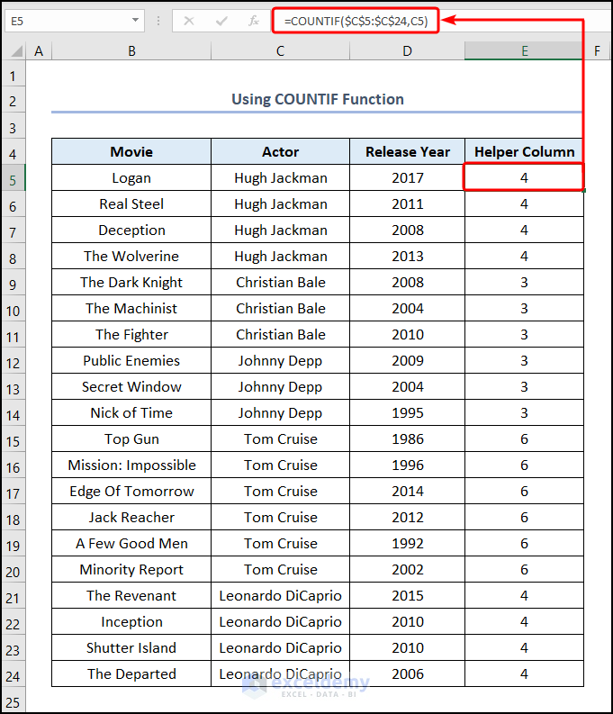
- Go to cell E5 and enter the formula written below.
=COUNTIF($C$5:$C$24,C5)
The C5:C24 range refers to the Actors column, and the C5 cell indicates the Hugh Jackman.
Formula Breakdown
- COUNTIF($C$5:$C$24,C5) → It counts the number of cells within a range that meet the given condition. Cells C5 to C24 represent the range argument that refers to the Actor, while the C5 cell indicates the criteria argument that returns the count of the matched value.
- Output → 4
Note: Please make sure to use Absolute Cell Reference by pressing the F4 key on your keyboard.
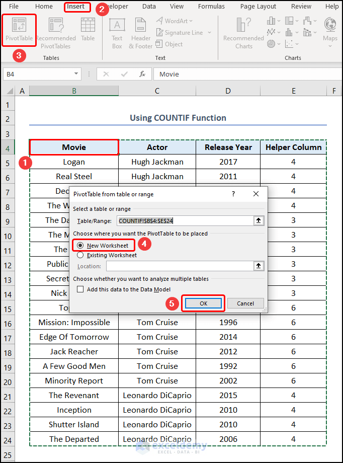
- Move to cell B5 cell and navigate to the Insert tab.
- Click on the PivotTable button.
- Check the New Worksheet box in the PivotTable pop-up window.
- Hit OK.
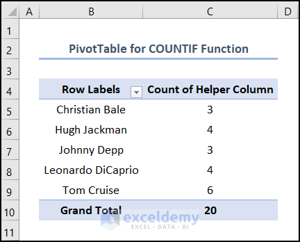
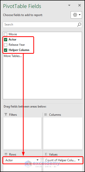
- Drag the Actor and Helper Column fields into the Rows and Values areas, respectively.

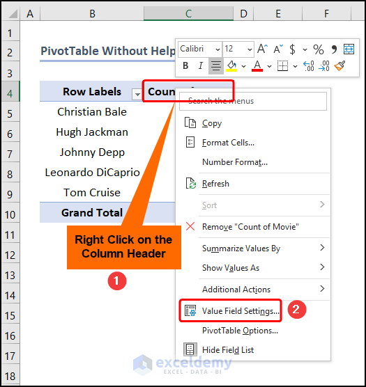
- Right-click on any of the column headers and press the Value Field Settings button.
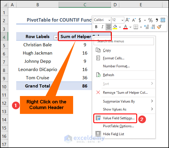
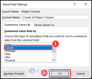
- Choose the Count option from the Summarize value field by list.
1.2 Combining the IF and COUNTIF Functions
Steps:
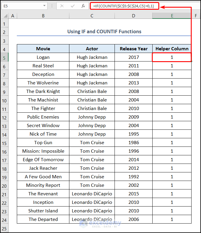
- Navigate to cell E5 and copy the following formula:
=IF(COUNTIF($C$5:$C$24,C5)>0,1)
Formula Breakdown
- IF(COUNTIF($C$5:$C$24,C5)>0,1) → Becomes
- IF(4>0,1) → Checks whether a condition is met and returns one value if TRUE and another value if FALSE. Here, 4>0 is the logical_test argument, which prompts the IF function to return “1” (value_if_true argument). Otherwise, it returns Blank (value_if_false argument).
- Output → 1
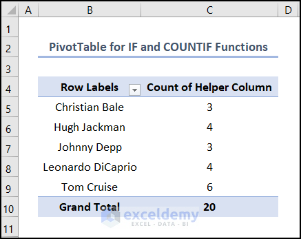
- Follow the steps outlined in the section above to insert the PivotTable and drag the fields into their respective locations.
The results should look like the image below.
1.3 Applying the IF and SUMPRODUCT Functions
Steps:
- Insert the following formula into the E5 cell:
=IF(SUMPRODUCT(($B$5:$B5=B5)*($C$5:$C5=C5))>1,0,1)
Formula Breakdown
- SUMPRODUCT(($B$5:$B5=B5)*($C$5:$C5=C5)) → Returns the sum of the products of the corresponding ranges or arrays. Here, the ($B$5:$B5=B5)*($C$5:$C5=C5) is the array1 argument where the value of the B5 and C5 cells is multiplied to give the output.
- Output → 1
- IF(SUMPRODUCT(($B$5:$B5=B5)*($C$5:$C5=C5))>1,0,1) → Becomes
- IF(1>1,0,1) → Here, 1>1 is the logical_test argument, which prompts the IF function to return “1” (value_if_true argument). Otherwise, it returns “0” (value_if_false argument).
- Output → 1
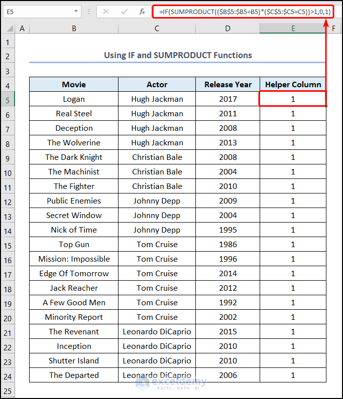
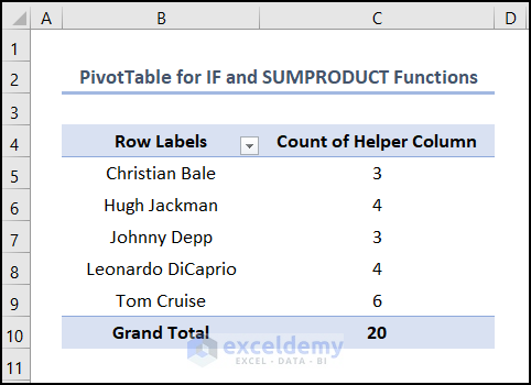
- Follow the steps shown previously to generate the output pictured below.
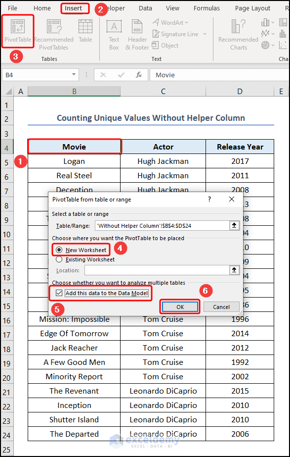
Method 2 – Counting Unique Values Without the Helper Column
Steps:
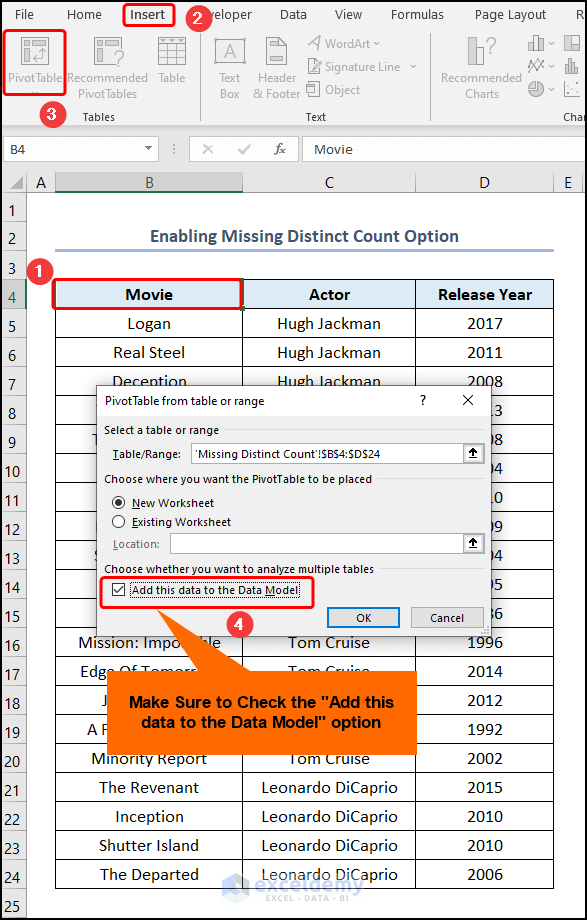
- Go to cell B5 and click on the Insert tab.
- Click on the PivotTable button.
- Enable the New Worksheet option and check the Add this data to the Data Model box.
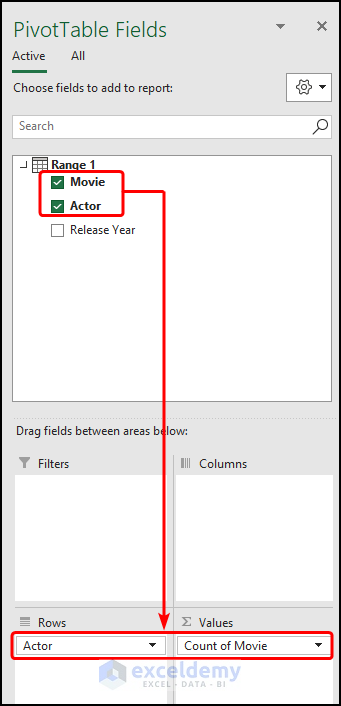
- Insert the Movie and Actor fields into the Rows and Values areas.
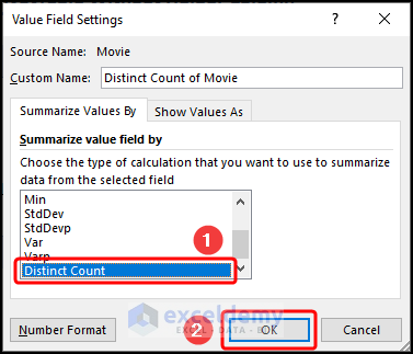
- Right-click on the column header and select the Value Field Settings option from the dropdown menu.
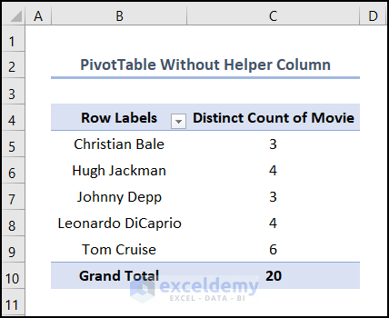
- Select the Distinct Count option and hit the OK button.

- The final output should look like the screenshot below.
Method 3 – Utilizing the PowerPivot Tool
Steps:
- Copy the data from the Dataset worksheet and paste it into the A1 cell of the Dataset for PowerPivot worksheet, as shown in the picture below.

- Open a new workbook, in this case, the Using PowerPivot.xlsx workbook.
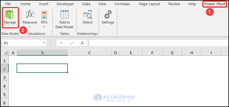
- Navigate to PowerPivot and click on the Manage option.
- Press the From Other Sources option.
- Choose the Excel File button and hit Next.

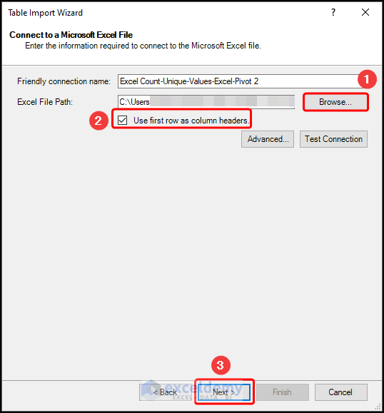
- Browse for the Excel file containing the Dataset for PowerPivot worksheet.
- Check the option to Use first row as column headers and press Next.
- Select the Dataset for PowerPivot worksheet and click on Finish.
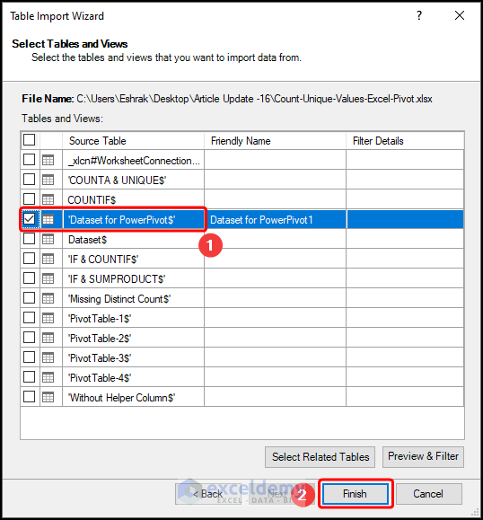
- Select the PivotTable option from the dropdown menu.
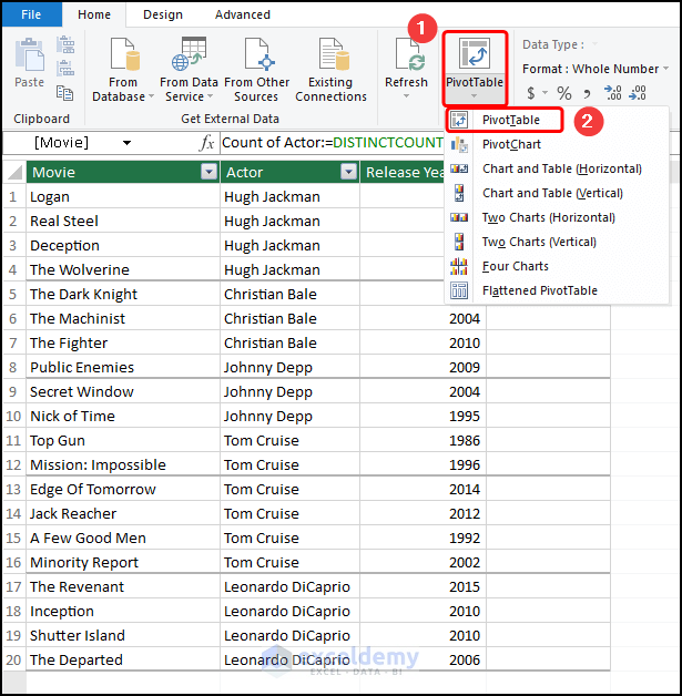
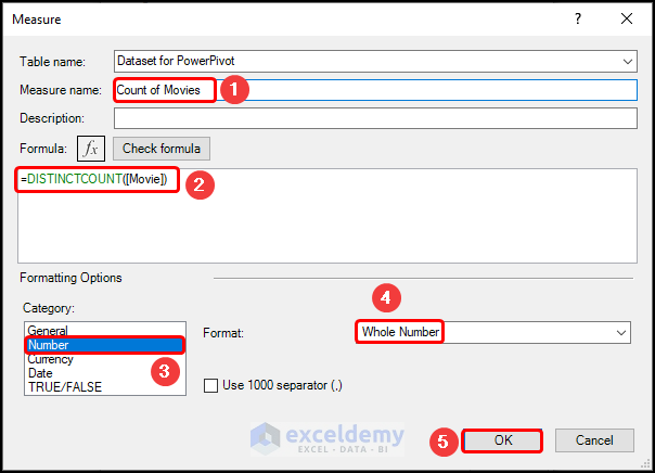
- In the PowerPivot tab, go to the Measures tab and launch the New Measure dropdown menu.

- Enter a Measure name, such as Count of Movies.
- Copy and paste the formula given below in the Formula field:
=DISTINCTCOUNT([Movie])
- Choose the Number option under the Category section.
- Format the value as a Whole Number.
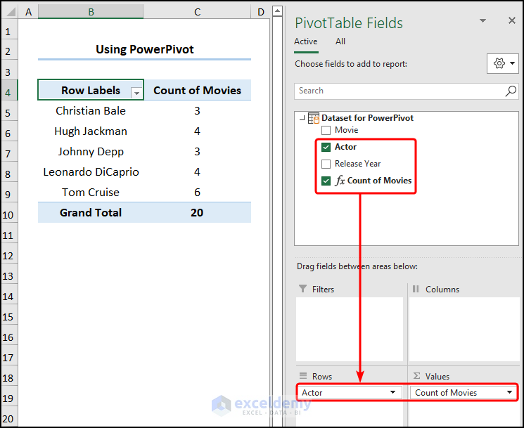
- Click on the Count of Movies measure.
- The final output should look like the image below.
Read More: Count Rows in Group with Pivot Table in Excel
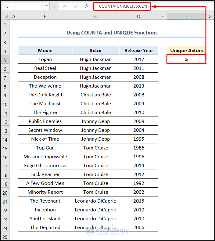
How to Count Unique Values With the COUNTA and UNIQUE Functions in Excel
Steps:
- Navigate to cell F5 and insert the formula below into the Formula Bar.
=COUNTA(UNIQUE(C5:C24))
In this example, the C5:C24 range refers to the Actor column.
Formula Breakdown
- UNIQUE(C5:C24) → Returns the unique values from a range or array. Here, the C5:C24 is the array argument that refers to the Actor column.
- Output → {“Hugh Jackman”;”Christian Bale”;”Johnny Depp”;”Tom Cruise”;”Leonardo DiCaprio”}
- COUNTA(UNIQUE(C5:C24)) → Counts the number of cells in a range that are not empty. Here, the UNIQUE(C5:C24) is the value1 argument that refers to the array returned by the UNIQUE function
- Output → 5
How to Enable the Missing Distinct Count Option of a Pivot Table in Excel
Steps:
- Insert a PivotTable as usual.
- Check the Add this data to the Data Model option.
- Open the Value Field Settings and locate the Distinct Count option in the Summarize value field by list.
Practice Section
There’s a Practice section on the right side of each sheet, so you can practice on your own.

Download Practice Workbook
<< Go Back to Pivot Table Count | Pivot Table Calculations | Pivot Table in Excel | Learn Excel
Get FREE Advanced Excel Exercises with Solutions!

Count Unique Values Using Excel Pivot Table without Helper Column was very helpful, thank you! This was a very simple and easy way to get the counts I needed. (Senior Analyst, Reporting and Metrics, Cardinal Health)
Thanks for commenting Merle, glad to hear that it helped you.
This feature doesn’t exist, i’m on the latest excel and its not there.
Bob, PivotTable is one of the prime features of Excel, so regardless of the version (contemporary versions) you should get it inside the “Insert” tab of the ribbon. But if you don’t find that there you may need to customize your ribbon. Click on File > Options, then follow the image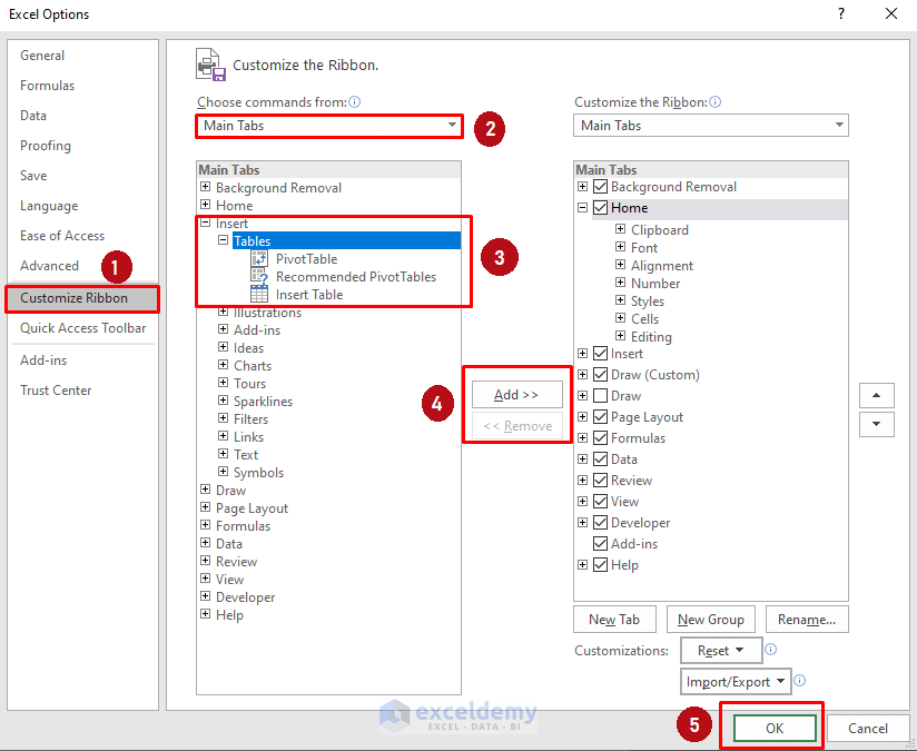
And if counting unique is your main goal right now you might get that using the UNIQUE function (and COUNT family function for counting).