Count Rows in Group with Pivot Table in Excel (Step-by-Step Guideline)

This article will guide you to count rows from a data group using Pivot Table. If you have a large dataset containing values in groups, you may be required to count rows in each group. Unfortunately, in Microsoft Excel, you cannot use formulas to calculate rows in a group. In such a case, the Pivot Table is a great way to calculate the count of rows from groups.

What is Pivot Table in Excel

Pivot Table is one of the most powerful tools available in Excel. If you are working with large datasets and have no clue what that data means, Pivot Tables enable you to understand the patterns of the data. You can understand the trends of data by analyzing them with the Pivot Table. Besides, we can group data in different ways using Pivot Tables. Later, from these data groups, we can draw effective conclusions too. To summarize, Pivot Tables enable us to get meaningful information from a large amount of random data.

Count Rows in Group with Pivot Table in Excel: Step-by Step Procedure

Dataset Introduction

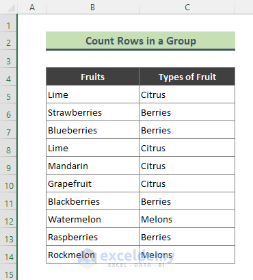
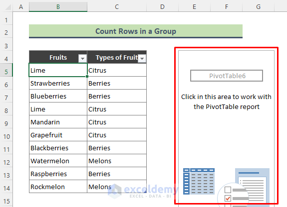
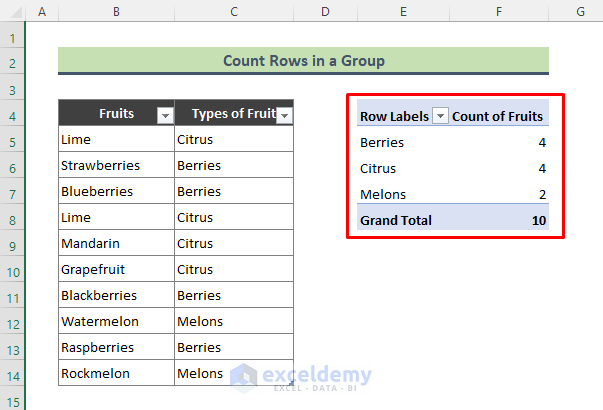
Let’s assume we have a dataset containing several fruits and their corresponding fruit types. Now, I will find out the number of rows in each group of fruit types. For instance, I will calculate the number of rows from column B that contain fruits from the Citrus/Melon/Berries group.

Step 1: Insert Excel Pivot Table to Count Rows in Group

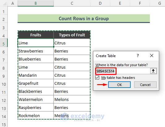
• Before inserting the Pivot Table, I will convert my dataset into a Defined Table by pressing Ctrl + T.

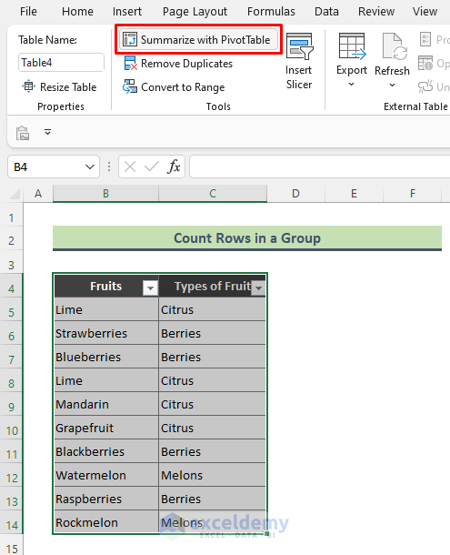
• After you get the table, click Summarize with PivotTable option.

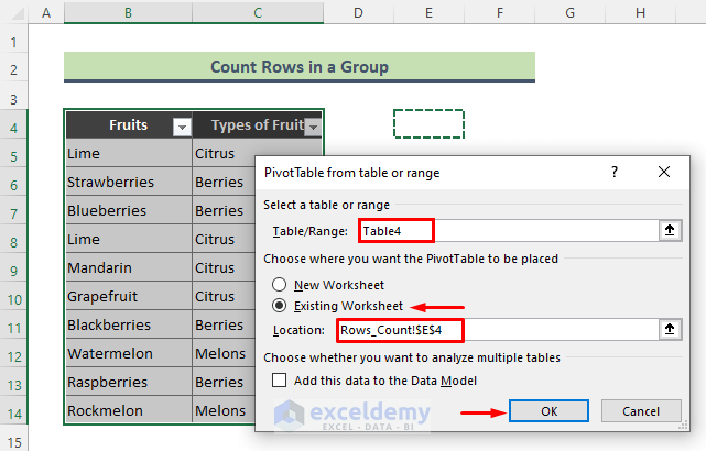
• As a result, the PivotTable from table or range dialog box appears. Now, check the Table/Range and choose the location where you want to place the Pivot Table as below (see the screenshot). I want to place the Pivot Table in the existing worksheet (cell E4). After choosing the Location, press OK.

• Consequently, you will get the below Pivot Table.

⏩ Note:

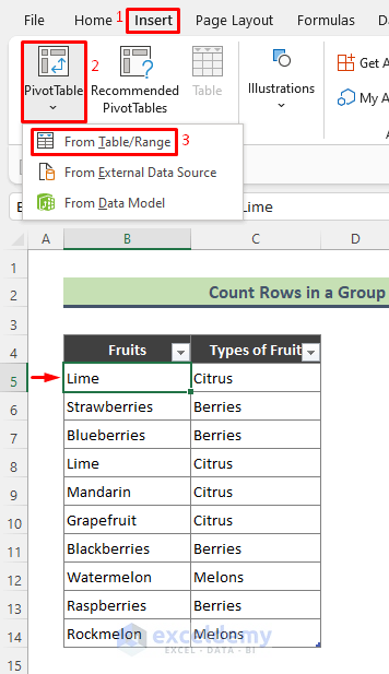
You can insert Pivot Table by following the path: Insert > Pivot Table > From Table/Range

Step 2: Get the Rows Count in a Group from Pivot Table

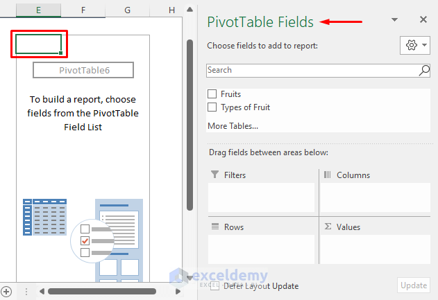
Now, I will customize the newly created Pivot Table according to my requirements. To do the task, follow the below instructions.

• Click on the Pivot Table area to show the PivotTable Fields section.

• Next, drag the Types of Fruit field to the Rows area. Similarly, drag Fruits to the Values area.

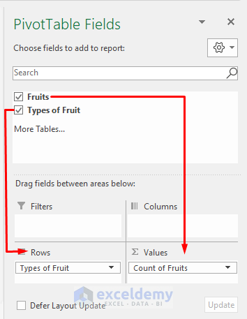
• Finally, we got the count of rows under each type of fruit. From the result, we can see that the Berries and Citrus group has fruits in 4 rows. On the other hand, there are 2 rows in the Melons group.

Things to Remember

• It is better to convert the existing data range to an Excel table before inserting the Pivot Table. This is because if you add any new data to the source table, refreshing the Pivot Table will update the Pivot Table data too.
• You can count unique values using Pivot Tables (by adding a Helper column in the source dataset). Likewise, you can use Power Pivot to calculate the unique count of values in a dataset.

Download Practice Workbook

You can download the practice workbook that we have used to prepare this article.

Conclusion

In the above article, I have tried to discuss step-by-step guidelines to count rows in a group with Pivot Table in Excel. Hopefully, these methods and explanations will be enough to solve your problems. Please let me know if you have any queries.

<< Go Back to Pivot Table Count | Pivot Table Calculations | Pivot Table in Excel | Learn Excel