How to Create a Percentage Progress Bar in Excel (3 Methods)

A percentage progress bar is a powerful visual tool that allows you to compare working rates, track task statuses, and understand information instantly. In this article, I’ll guide you through three methods to create a percentage progress bar in Excel to compare the working rates of different teams.

Let’s use the following dataset: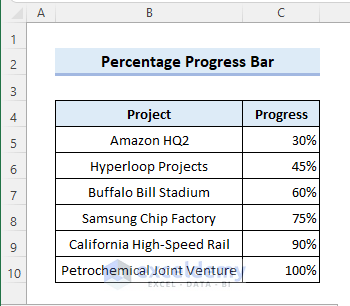

Method 1 – Using a Bar Chart

You can show the percentage progress bar by inserting a Bar Chart in Excel. Follow the steps below to do that.

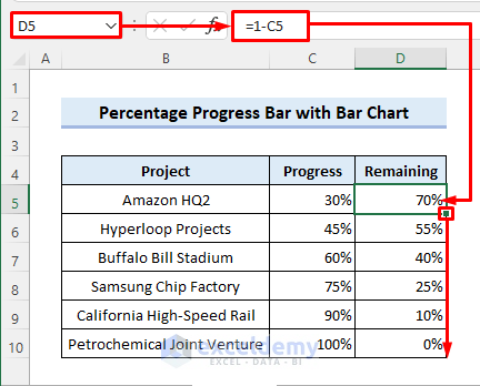
• Enter the Formula:
  • Start by opening your Excel workbook and locating the dataset where you want to display the progress bar.
  • In cell D5 (or any other cell within the data range), enter the following formula:

This formula calculates the percentage completion based on the values in cells B5 (completed tasks) and C5 (total tasks). Adjust the cell references according to your dataset.

• Copy the Formula:
  • Drag the Fill Handle icon (a small square at the bottom-right corner of the cell) down to copy the formula to the cells below (D6, D7, etc.). This will calculate the percentage for each row in your dataset.

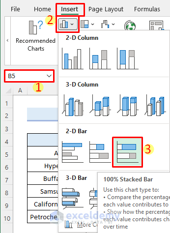
• Insert a Bar Chart:
  • Select any cell within the data range.
  • Go to the Insert tab in the Excel ribbon.
  • Choose Column or Bar Chart from the Charts group.
  • Select the 100% Stacked Bar chart type from the 2-D Bar options.

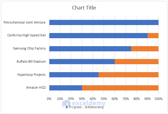
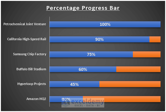
After following the steps mentioned above, the 100% Stacked Bar chart will be inserted into your Excel workbook. This chart will visually represent the progress percentage for different tasks or teams.

• Customize the Chart:
  • The 100% Stacked Bar chart will display the percentage completion for each data point.
  • Customize the chart by adjusting labels, colors, and other formatting options to make it visually appealing.
  • You can also add a title and axis labels to provide context.

• Result:
  • Your percentage progress bar chart will now show the progress of different tasks or teams.

Remember to adapt these steps to your specific dataset and preferences. With this method, you’ll have an informative progress bar that visually represents your data in Excel!

Method 2 – Using Data Bars

• Select the Range:
  • Highlight the entire range (C5:C10) that contains the progress percentages.

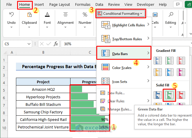
• Apply Data Bars:
  • Go to the Home tab in Excel.
  • Click on Conditional Formatting and choose Data Bars.
  • Select your desired fill color (either from Gradient Fill or Solid Fill options).

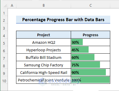
• Adjust Text Alignment:
  • Make sure the text within the cells is left-aligned.
  • This will display the data bars alongside the percentage values.

Method 3 – Using the Excel REPT Function

• Select Cell D5:
  • Click on cell D5 where you want to display the progress bar.

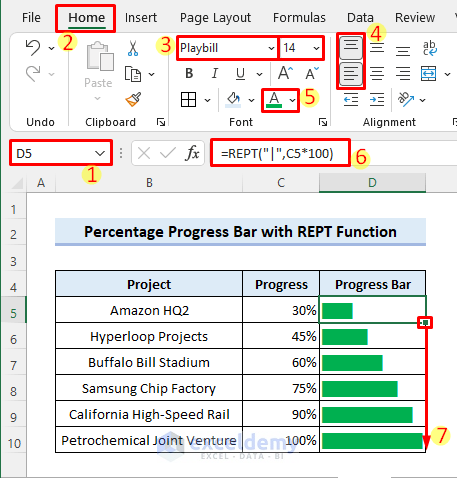
• Customize Font and Alignment:
  • Change the font to Playbill from the Home tab.
  • Choose top and left alignments for the cell.

• Set Fill Color:
  • Select a fill color for the cell (you can use the same color as the data bars).

• Enter the Formula:
  • In cell D5, enter the following formula:

This formula repeats the “|” character based on the percentage value in cell C5.

• Copy the Formula:
  • Drag the Fill Handle icon down to copy the formula to other cells (D6, D7, etc.).

• Result:
  • You’ll see a vertical progress bar made of “|” characters, representing the progress percentage.

Things to Remember

• Customize the 100% Stacked Bar chart (from Method 1) as needed.
• You can also apply data bars directly to cells using conditional formatting.

Download Practice Workbook

You can download the practice workbook from here:

Related Articles

• How to Create Progress Bar Based on Another Cell in Excel
• Progress Bar in Excel Cells Using Conditional Formatting

<< Go Back to Progress Bar in Excel | Data Visualisation in Excel | Learn Excel