How to Reference Pivot Table Data in Excel (with Easy Steps)

Get FREE Advanced Excel Exercises with Solutions!

In this article, I have shown you how you can reference Pivot Table data in Excel formulas using the GETPIVOTDATA function. If you feel uneasy with the auto implementation of the GETPIVOTDATA function in the Excel formulas, you can stop it!

After you have created a pivot table, you may want to create formulas that will reference one or more cells within that pivot table. Here is the way how you can do that.


What Is Pivot Table Reference?

Pivot Table referencing means to take value from the pivot table to another cell. Sometimes you need to take some specific data from the pivot table. In that case, referencing is essential. The Pivot table helps you to narrow down a large dataset and establish a relationship between data points. It recognizes the dataset metrics and dimensions and provides a meaningful summary of it. After creating the pivot table, you may have needed to reference it to another cell or new worksheet. In that case, you can use the GETPIVOTDATA function. But you can use direct cell reference, but in that case, if you alter the pivot table format, the cell will show an error. Whereas, the GETPIVOTDATA function won’t give any error.


How to Reference Pivot Table Data in Excel: Step-by-Step Procedures

Before referencing pivot table data using the GETPIVOTDATA function, we need to take a dataset and convert it into the pivot table. After that, we want to use the GETPIVOTDATA function and get the desired result. To understand the process clearly, follow the steps.


Step 1: Creating Pivot Table

Our first step is to create a pivot table using the existing dataset. After making the required pivot table, you can reference the pivot table for other purposes. Follow the process.

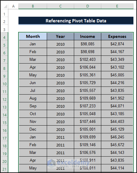
  • First, select the range of cells B4 to E40.

Creating Pivot Table to Reference Pivot table Data in Excel

  • Then, go to the Insert tab in the ribbon.
  • After that, select PivotTable from the Tables group.

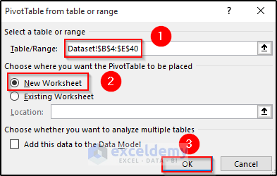
  • Then, the PivotTable from table or range dialog box will appear.
  • Select the range of cells.
  • Then, choose where you want to place your Pivot Table.
  • Finally, click on OK.

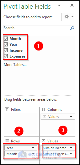
  • As a consequence, you will see a PivotTable Fields dialog box will appear.
  • Then, check all the options first.
  • After that, drag the month and year in the Rows section and income and expense in the Values section.

Making Pivot Table to Reference Pivot table Data in Excel

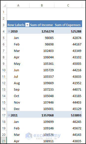
  • As a result, we will get the required pivot table. See the screenshot.


Step 2: Calculate Ratio of Expenses and Income for Three Different Years

In this step, we would like to calculate the ratio of expenses and income for three different years. To do this, we will utilize the GETPIVOTDATA function. To understand this carefully, follow the steps.

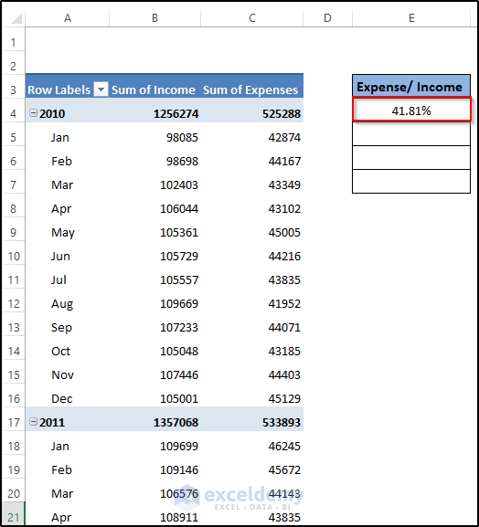
  • First, we would like to take expenses and income for the year 2010.
  • Select cell E4.
  • Then, write down the following formula.

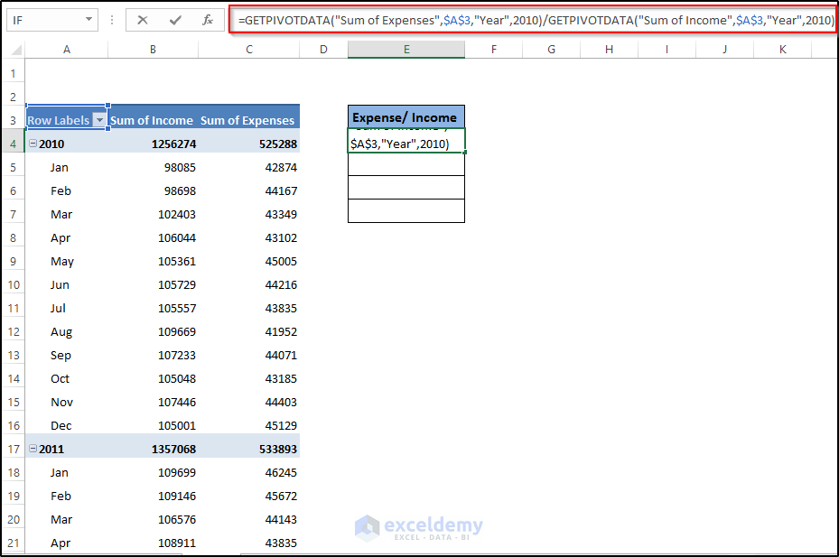
=GETPIVOTDATA("Sum of Expenses",$A$3,"Year",2010)/GETPIVOTDATA("Sum of Income",$A$3,"Year",2010)

  • As writing this formula is a tedious process, you can do it in another easy way.
  • First, select cell E4.
  • Then, press the equal(=) sign there.
  • After that, click on the sum of expenses for 2010 in the pivot table.
  • Then, use the divide(/) sign.
  • After that, click on the sum of income for 2010 in the pivot table.
Calculate Ratio of Expenses and income by Referencing Pivot Table

  • Finally, press Enter to apply the formula.

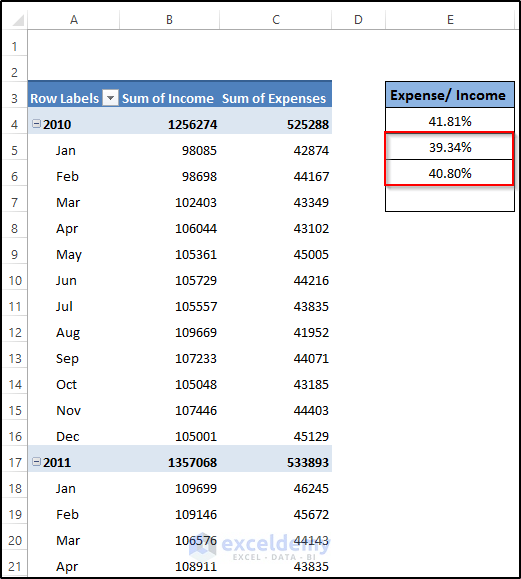
  • After that, do the same procedure to get the ratio of expenses and income for the years 2011 and 2012.
  • Finally, you will get the following result. See the screenshot.

Estimate Ratio of Expenses and income by Referencing Pivot Table


Step 3: Calculate Overall Ratio of Expenses and Income

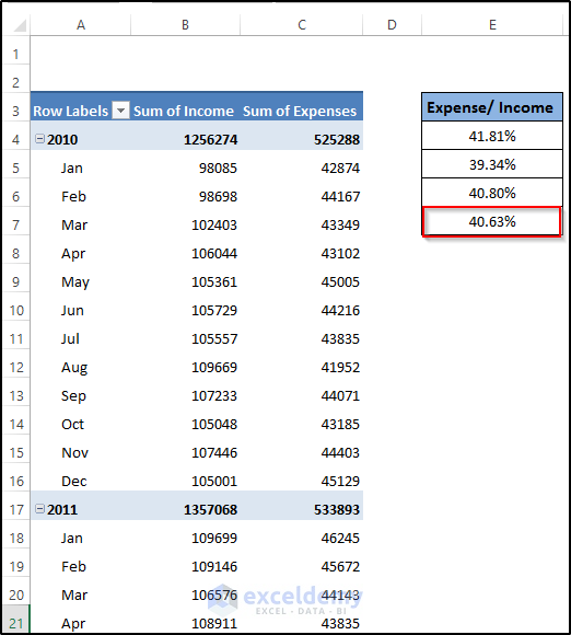
In this step, we would like to calculate the overall ratio of expenses and income. for all three years. To do this, we will use the use the GETPIVOTDATA function. Because of the pivot table, we get the total at the end of the pivot table. Follow the steps.

  • First, select cell E7.
  • Then, write down the following formula.
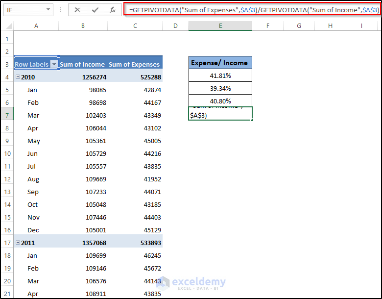
=GETPIVOTDATA("Sum of Expenses",$A$3)/GETPIVOTDATA("Sum of Income",$A$3)
  • As writing this formula is a tedious process, you can do it in another easy way.
  • First, select cell E7.
  • Then, press the equal(=) sign there.
  • After that, click on the grand total of the sum of expenses in the pivot table.
  • Then, use the divide(/) sign.
  • After that, click on the grand total of the sum of income in the pivot table.
Calculate Overall Ratio of Expenses and Income by Referencing Pivot Table

  • Then, press Enter to apply the formula.

Caution: Using the GETPIVOTDATA function has one limitation: The data that it retrieves must be visible. If you modify the pivot table so that the value used by GETPIVOTDATA is no longer visible, the formula will return an error.


How to Stop Auto-Using GETPIVOTDATA Function

If you want to prevent Excel from using the GETPIVOTDATA function when you point to pivot table cells at the time of creating a formula, you can do it using two different Ways.


1. Using PivotTable Analyze

We can quickly stop auto-using the GETPIVOTDATA function by using the PivotTable analyze tab on the ribbon. To apply this, follow the steps.

Steps

  • To enable the PivotTable analyze tab on the ribbon, you need to select any cell in the pivot table.
  • Then, you will see the PivotTable analyze tab.
  • Select the PivotTable analyze tab on the ribbon.
  • Then, select the Options drop-down option from the Pivot Table group.
  • After that, uncheck the Generate GetPivotData option.


2. Utilizing Excel Options

Another way you can stop auto-using the GETPIVOTDATA function is by utilizing Excel options. After unchecking the GetPivotData option, you can stop auto-using the GETPIVOTDATA function. Follow the steps.

Steps

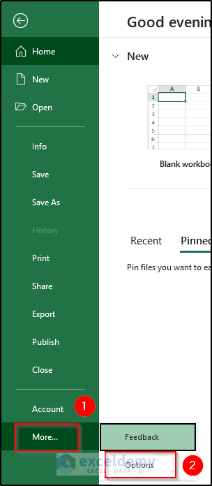
  • First, go to the File tab on the ribbon.
  • Then, select the More command.
  • After that select Options.

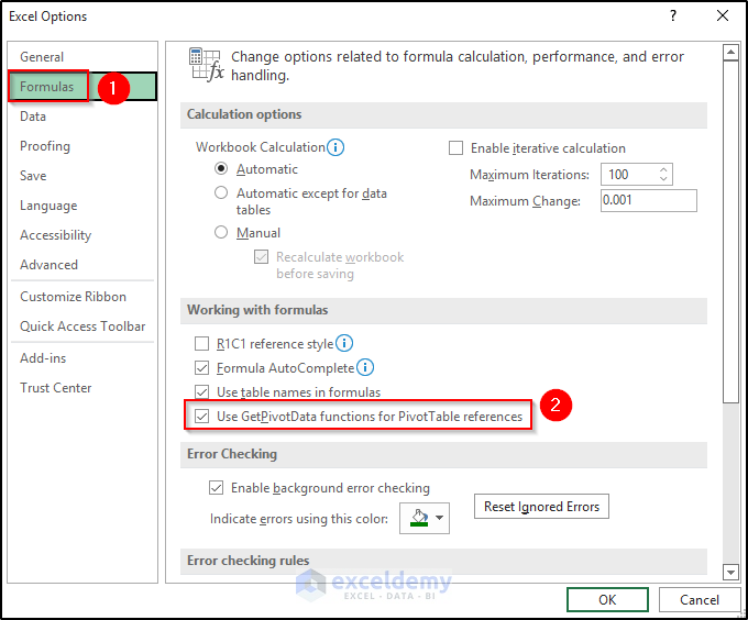
  • It will open up the Excel Options dialog box.
  • Then, select the Formulas option.
  • After that, uncheck the Use GetPivotData functions for PivotTable references from the Working with formulas section.
  • Finally, click on OK.


Things to Remember

  • Even if you change the layout of the pivot table, the GETPIVOTDATA function shows the correct result. But in the case of only a cell reference, it returns an error if you modify the layout.
  • Excel produces the GETPIVOTDATA function in that way if you click on the pivot table, it will take it as a formula.

Download Practice Workbook

Download the practice workbook below.


Conclusion

We have shown step-by-step procedures to do referencing in the pivot table. All of these steps are fairly easy to understand. To do referencing in the pivot table, we utilize the GETPIVOTDATA function. In this article, we also include how to stop auto-using the GETPIVOTDATA function. I hope we covered all possible areas of this topic. If you have any questions, feel free to ask in the comment section.


<<Go Back to Excel GETPIVOTDATA | Pivot Table in Excel | Learn Excel

What is ExcelDemy?

ExcelDemy - Learn Excel & Get Excel Solutions Center provides online Excel training , Excel consultancy services , free Excel tutorials, free support , and free Excel Templates for Excel professionals and businesses. Feel free to contact us with your Excel problems.
Kawser Ahmed
Kawser Ahmed

Kawser Ahmed is a Microsoft Excel Expert, Udemy Course Instructor, Data Analyst, Finance professional, and Chief Editor of ExcelDemy. He is the founder and CEO of SOFTEKO (a software and content marketing company). He has a B.Sc in Electrical and Electronics Engineering. As a Udemy instructor, he offers 8 acclaimed Excel courses, one selected for Udemy Business. A devoted MS Excel enthusiast, Kawser has contributed over 200 articles and reviewed thousands more. His expertise extends to Data Analysis,... Read Full Bio

4 Comments
  1. I have referenced few cells of the pivot table in another file. Whenever I open that other file containing reference, I see “#REF#” in the cells where I have references to the pivot table. As soon as I’ll open the file containing the pivot table, those cells would automatically populate the correct data. How can I fix this problem, so that I don’t have to open multiple files to see the data in my report?

  2. How do I reference a cell on another tab in the main pivot cell? When using =. . . I get the following error: ‘Cannot enter a formula for an item or field name in a PivotTable report’

    • Hi GENOBLE,
      Your question is greatly appreciated. You can easily fix your error by enabling Excel’s GetPivot Data function. If you want to enable Excel to use the GETPIVOTDATA function when you point to pivot table cells at the time of creating a formula, choose PivotTable Tools Analyze PivotTable Options Generate GetPivot Data command. Now, you can easily reference a cell on another tab in the main pivot cell.

Leave a reply

Advanced Excel Exercises with Solutions PDF


ExcelDemy
Logo