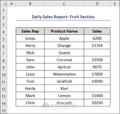
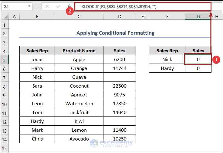
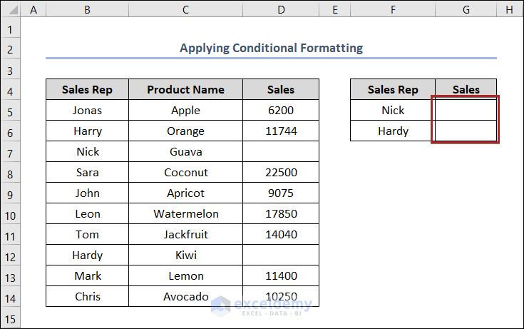
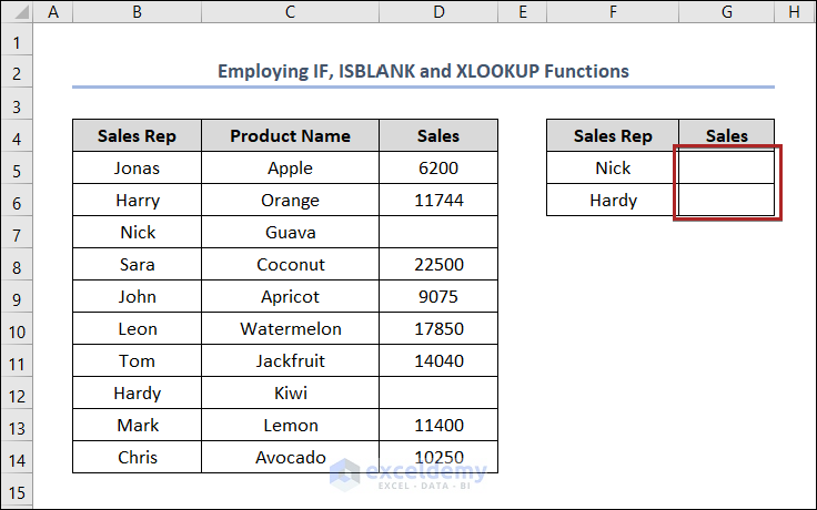
How to Use XLOOKUP to Return Blank Instead of 0 -12 Methods

The following dataset contains the names of Sales Reps, Product Names, and Sales.

Method 1 – Utilizing an Optional Argument of the XLOOKUP Function

Steps

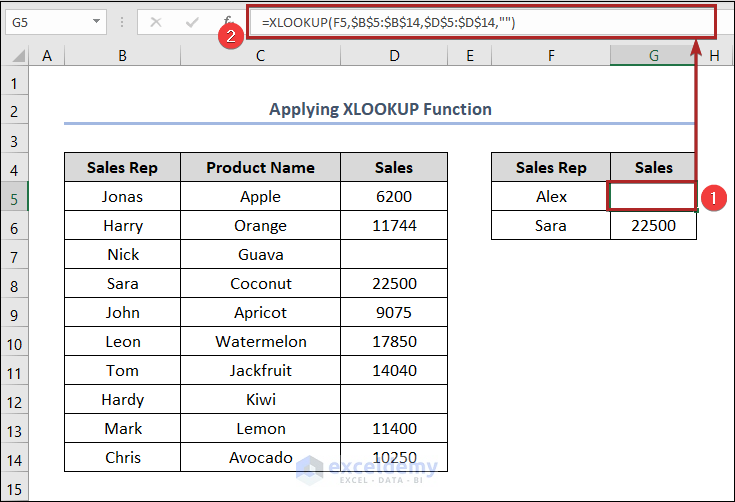
Select G5.
Enter the formula below.

=XLOOKUP(F5,$B$5:$B$14,$D$5:$D$14,"")

Formula Breakdown
Here, F5 represents the lookup_value (Alex).
B5:B14 is the lookup_array (the names of the Sales Rep).
D5:D14 is the return_array (Sales amount).
We used “” for [if_not_found]. If the function can’t find any matches, it will return blank.
The dollar (﹩) sign is used to provide an absolute reference.

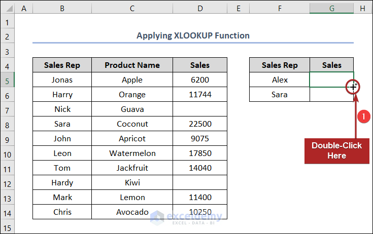
Press ENTER.

Double-click the Fill Handle to copy the formula to cell G6.

One of the cells will be blank.

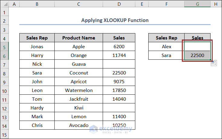
G6 contains the output because it’s present in Column B and has its respective Sales amount.

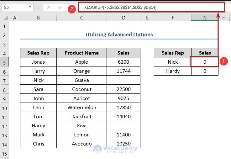
Method 2 – Using Advanced Options to Make XLOOKUP Return Blank Instead of 0

Steps

Select G5.
Enter the following formula in the Formula Bar.

=XLOOKUP(F5,$B$5:$B$14,$D$5:$D$14)

It’s the same formula used in Method 1.

Press ENTER.

Go to the File tab.

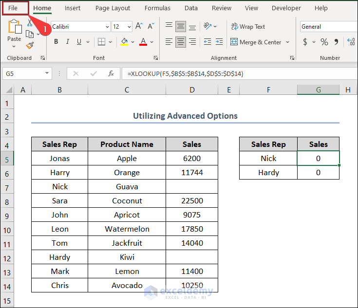
Select Options from the menu.

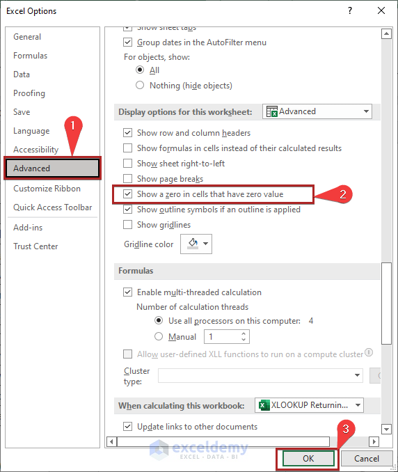
The Excel Options window will open.
Go to the Advanced tab.
Uncheck the box Show a zero in cells that have zero value under the section Display options for this worksheet.
Click OK.

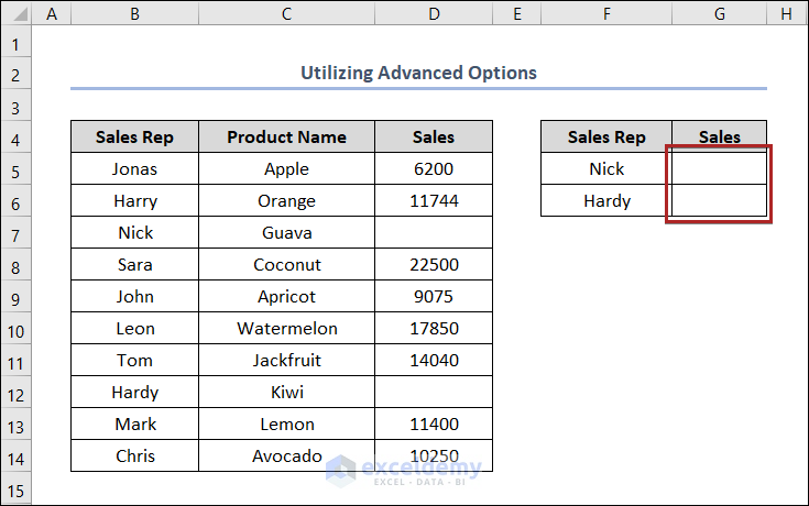
The two cells will be blank.

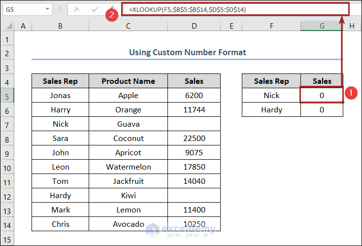
Method 3 – Using a Custom Number Format

Steps

Select G5.
Enter the following formula.

=XLOOKUP(F5,$B$5:$B$14,$D$5:$D$14)

It’s the same formula used in Method 1.

Press ENTER.

Select cells in the G5:G6 range.
Press CTRL+1.

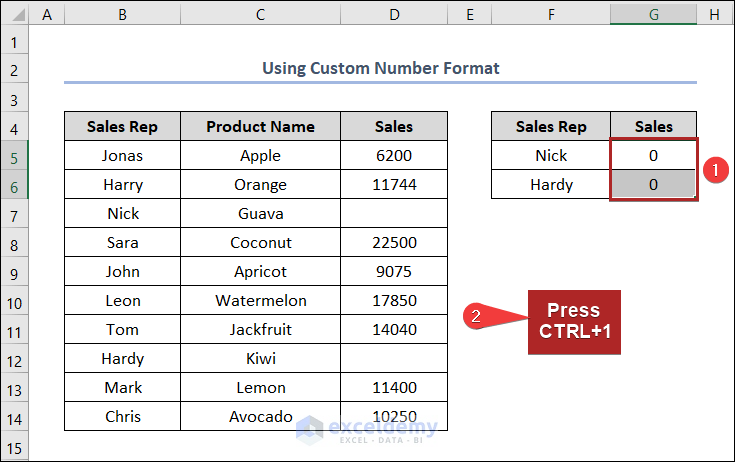
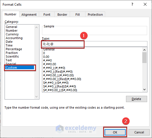
The Format Cells wizard will open.
In Category, select Custom.
in Type, enter 0;-0;;@.
Click OK.

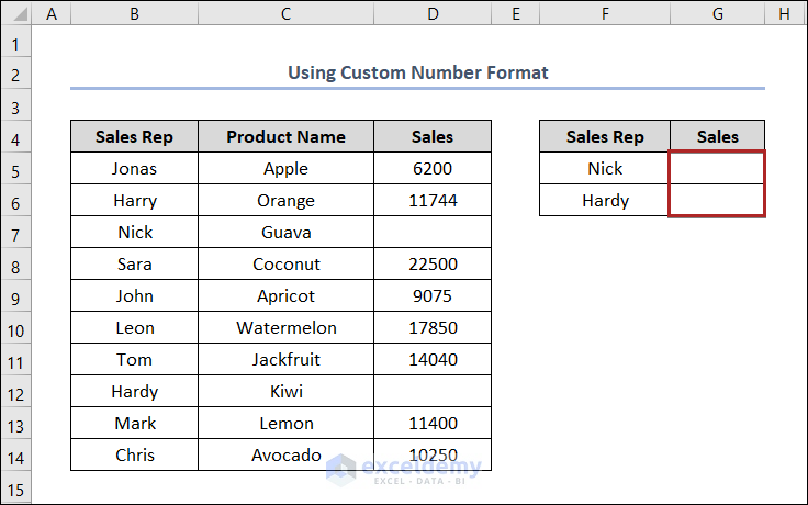
The two cells are blank in your worksheet.

Method 4 – Applying Conditional Formatting

Steps

Select cell G5 and enter the formula like in Method 1.

=XLOOKUP(F5,$B$5:$B$14,$D$5:$D$14,"")

Press ENTER.

Select cells in the B4:G14 range.
Go to the Home tab.
In Styles, select Conditional Formatting.
Choose New Rule from the drop-down list.

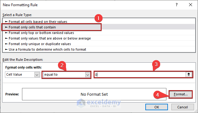
The New Formatting Rule dialog box will open.
In Select a Rule Type, choose Format only cells that contain.
Select equal to from the list.
Enter 0 in the box.
Click Format.

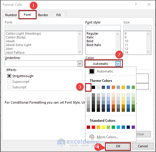
The Format Cells dialog box will open.
Go to the Font tab.
Select the Color from the drop-down list.
Choose White, Background 1.
Click OK.

The New Formatting Rule dialog box will be displayed again.
Click OK.

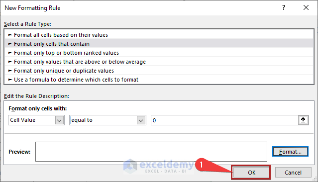
Cells are blank in the output.

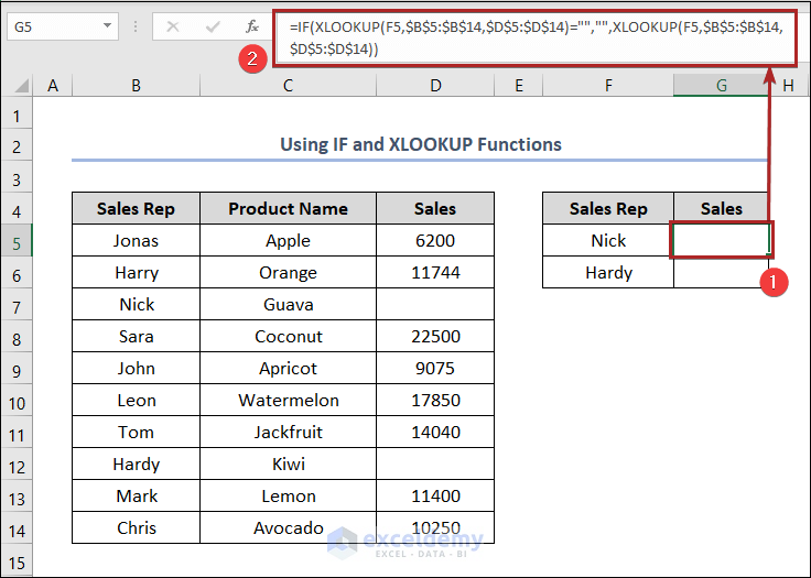
Method 5. Using the IF and XLOOKUP Functions to Return Blank Instead of 0

Steps

Select G5.
Enter the following formula in the cell.

=IF(XLOOKUP(F5,$B$5:$B$14,$D$5:$D$14)="","",XLOOKUP(F5,$B$5:$B$14,$D$5:$D$14))

Formula Breakdown
XLOOKUP(F5,$B$5:$B$14,$D$5:$D$14): looks for the value of cell F5 in your dataset, which is located in the range B5:B14, and inserts the corresponding value in the range D5:D14. As the value in Column D for the value of F5 is blank, the function will return 0. Otherwise, it will provide the value.

IF(XLOOKUP(F5,$B$5:$B$14,$D$5:$D$14)=””,””,XLOOKUP(F5,$B$5:$B$14,$D$5:$D$14)): checks the value of the XLOOKUP function. If the XLOOKUP function returns blank or the logic is true, the IF function returns blank in G5. If the logic is false, it returns the value of the XLOOKUP function.

Press ENTER.

A blank cell is displayed instead of 0.
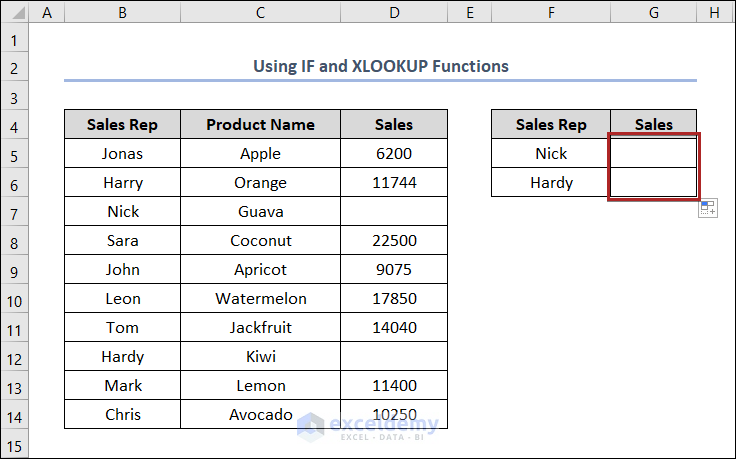
Double-click the Fill Handle to copy the formula to G6.

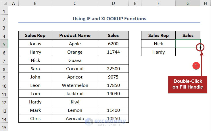
Blank cells will be displayed for the two values.

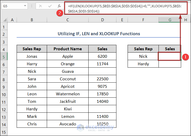
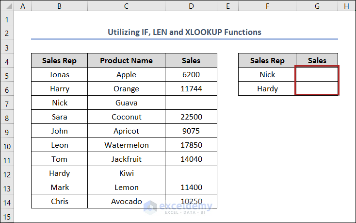
Method 6. Utilizing the IF, LEN, and XLOOKUP Functions

Steps

Select G5.
Enter the following formula in the cell.

=IF(LEN(XLOOKUP(F5,$B$5:$B$14,$D$5:$D$14))=0,"",XLOOKUP(F5,$B$5:$B$14,$D$5:$D$14))

Formula Breakdown
XLOOKUP(F5,$B$5:$B$14,$D$5:$D$14): looks for the value of F5 in your dataset, which is located in the range B5:B14, and it inserts the corresponding value in the range D5:D14. As the value in Column D for the value of F5 is blank, the function will return 0. Otherwise, it will provide the value.

LEN(XLOOKUP(F5,$B$5:$B$14,$D$5:$D$14)): counts the character length of the result obtained from the XLOOKUP function. Here, 0.

IF(LEN(XLOOKUP(F5,$B$5:$B$14,$D$5:$D$14))=0,””,XLOOKUP(F5,$B$5:$B$14,$D$5:$D$14)): checks the value of the LEN function. If the result of the LEN function is 0 or the logic is true, the IF function returns blank in G5. If the logic is false, it returns the value of the XLOOKUP function.

Press ENTER.

Drag the Fill Handle to get blank cells for the two values.

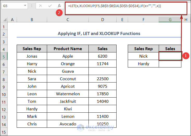
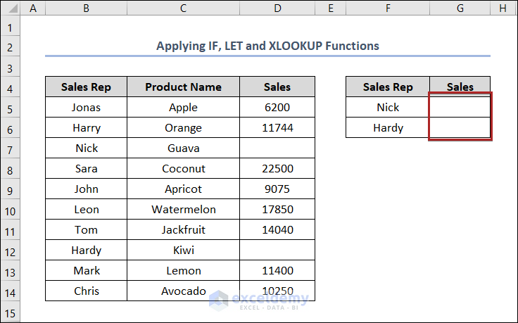
Method 7 – Applying the IF, LET, and XLOOKUP Functions to Return Blank Instead of 0

Steps

Select G5.
Enter the following formula in the cell.

=LET(x,XLOOKUP(F5,$B$5:$B$14,$D$5:$D$14),IF(x="","",x))

Formula Breakdown
XLOOKUP(F5,$B$5:$B$14,$D$5:$D$14): looks for the value of F5 in your dataset, which is located in the range B5:B14, and inserts the corresponding value in the range D5:D14. As the value in Column D for the value of F5 is blank, the function will return 0. Otherwise, it will provide the value.

LET(x,XLOOKUP(F5,$B$5:$B$14,$D$5:$D$14),IF(x=””,””,x)): creates a variable named x and uses the result from the XLOOKUP function to assign the value of x. With the IF function, If x is empty, an empty string (“”) is returned. Otherwise, it returns the value of x.

Press ENTER.

This is the output.

Method 8 – Using the IF, ISBLANK, and XLOOKUP Functions

Steps

Select G5 and enter the following formula.

=IF(ISBLANK(XLOOKUP(F5,$B$5:$B$14,$D$5:$D$14)),"",XLOOKUP(F5,$B$5:$B$14,$D$5:$D$14))

Formula Breakdown
XLOOKUP(F5,$B$5:$B$14,$D$5:$D$14): looks for the value of F5 in your dataset, which locates in the range B5:B14, and inserts the corresponding value in the range D5:D14. As the value in Column D for the value of F5 is blank, the function will return 0. Otherwise, it will provide the value.

ISBLANK(XLOOKUP(F5,$B$5:$B$14,$D$5:$D$14)): checks the result from the XLOOKUP function. If the cell is empty the function will return TRUE. Otherwise, it will return FALSE. In this case, the value is TRUE.

IF(ISBLANK(XLOOKUP(F5,$B$5:$B$14,$D$5:$D$14)),””,XLOOKUP(F5,$B$5:$B$14,$D$5:$D$14)): checks the value of the ISBLANK function. If the result of the ISBLANK function is true, the IF function returns blank in G5. If the logic is false, the function returns the value of the XLOOKUP function.

Press ENTER.

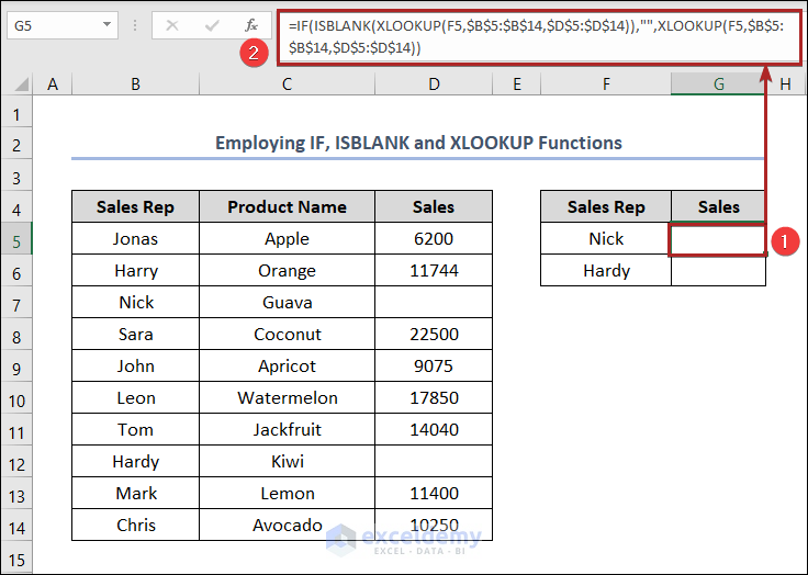
This is the final output.

Method 9 – Using the IF, ISNUMBER, and XLOOKUP Functions to Return Blank Instead of 0

Steps

Select G5.
Enter the following formula.

=IF(ISNUMBER(XLOOKUP(F5,$B$5:$B$14,$D$5:$D$14)),XLOOKUP(F5,$B$5:$B$14,$D$5:$D$14),"")

Formula Breakdown
XLOOKUP(F5,$B$5:$B$14,$D$5:$D$14): looks for the value of F5 in your dataset, which locates in the range B5:B14, and it inserts the corresponding value in the range D5:D14. As the value in Column D for the value of F5 is blank, the function will return 0. Otherwise, it will provide the value.

ISNUMBER(XLOOKUP(F5,$B$5:$B$14,$D$5:$D$14)): checks the result from the XLOOKUP function. If the cell is empty the function will return FALSE. Otherwise, it will return TRUE. In this case, the value is FALSE.

IF(ISNUMBER(XLOOKUP(F5,$B$5:$B$14,$D$5:$D$14)),XLOOKUP(F5,$B$5:$B$14,$D$5:$D$14),””): checks the value of the ISNUMBER function. If the result of the ISNUMBER function is FALSE, the IF function returns blank in G5. If the logic is TRUE, it returns the value of the XLOOKUP function.

Press ENTER.

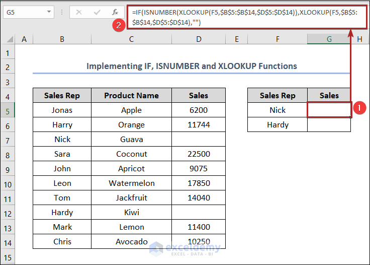
This is the final output.

Method 10 – Combining the IF, IFNA, and XLOOKUP Functions

Steps

Select cell G5.
Enter the following formula in the cell.

=IF(IFNA(XLOOKUP(F5,$B$5:$B$14,$D$5:$D$14),0)=0,"",XLOOKUP(F5,$B$5:$B$14,$D$5:$D$14))

Formula Breakdown
XLOOKUP(F5,$B$5:$B$14,$D$5:$D$14): looks for the value of cell F5 in your dataset, which locates in the range B5:B14, and inserts the corresponding value in the range D5:D14. As the value in Column D for the value of F5 is blank, the function will return 0. Otherwise, it will provide the value.

IFNA(XLOOKUP(F5,$B$5:$B$14,$D$5:$D$14),0): counts the character length of the result obtained from the XLOOKUP function. In this case, the value is 0.

IF(IFNA(XLOOKUP(F5,$B$5:$B$14,$D$5:$D$14),0)=0,””,XLOOKUP(F5,$B$5:$B$14,$D$5:$D$14)): checks the value of the IFNA function. If the result is 0, the IF function returns blank in G5. Otherwise, the function returns the value of the XLOOKUP function.

Press ENTER.

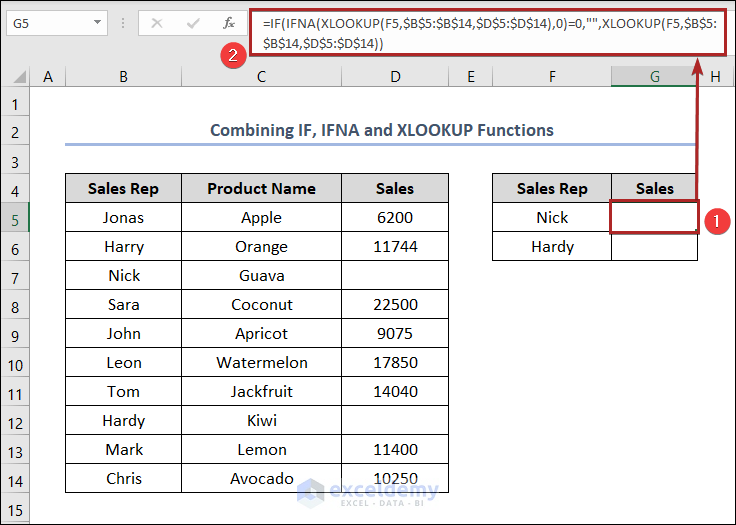
This is the final output.

Method 11. Using the IFERROR and the XLOOKUP Functions

Steps

Select G5.
Enter the following formula in the cell.

=IFERROR(XLOOKUP(F5,$B$5:$B$14,$D$5:$D$14),"")

IFERROR(XLOOKUP(F5,$B$5:$B$14,$D$5:$D$14),””): checks the value of the XLOOKUP function. If the result of the XLOOKUP function is 0, the IFERROR function returns blank in G5. Otherwise, the function returns the value of the XLOOKUP function.

Press ENTER.

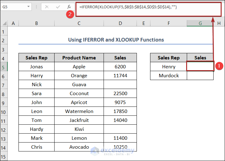
This is the output.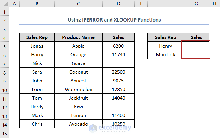

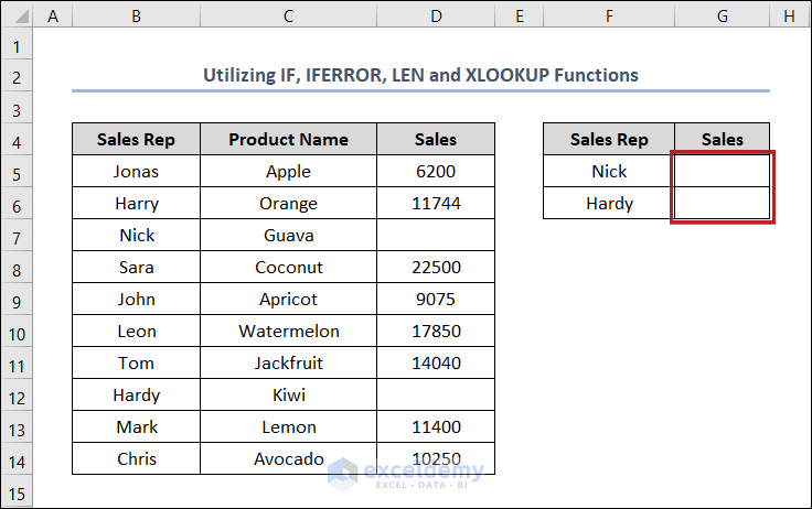
Method 12 – Utilizing the IF, IFERROR, LEN, and XLOOKUP Functions to Return Blank Instead of 0

Steps

Select G5.
Enter the following formula in the cell.

=IFERROR(IF(LEN(XLOOKUP(F5,$B$5:$B$14,$D$5:$D$14))=0,"",XLOOKUP(F5,$B$5:$B$14,$D$5:$D$14)),"")

LEN(XLOOKUP(F5,$B$5:$B$14,$D$5:$D$14)): counts the character length of the result obtained from the XLOOKUP function. In this case, the value is 0.

IFERROR(IF(LEN(XLOOKUP(F5,$B$5:$B$14,$D$5:$D$14))=0,””,XLOOKUP(F5,$B$5:$B$14,$D$5:$D$14)),””): checks the decision of the IF function. If the function returns a blank cell, the IFERROR function shows us the blank. Otherwise, it will show the value of the corresponding cell in Column D.

Press ENTER.

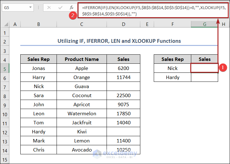
This is the output.

Practice Section

Practice here.

Download Practice Workbook

Download the following Excel workbook to practise.

XLOOKUP Returning Blank.xlsx

Get FREE Advanced Excel Exercises with Solutions!

2 Comments

Siam A. Sep 18, 2022 at 7:47 PM

First of all, many many thanks for this piece of writing. You have explained all the items in details.
A few days ago I was trying to solve a problem, but couldn’t.
This is like: in column A, i have A,B,C,B,A,C,B,A,C in order. Like A is in cell A1, B is in cell B2 and just like that. In column B, i’ve their respective value. These are like 180,360,200,400,203,350,160,500,233. From the above informations, iwant to find the minimum values of A.B,C.
I have tried using vlookup, but it can’t get the correct answer.
Would you please enlighten me how I can get the min value?
TIA
- Reply
  Shahriar Sep 19, 2022 at 12:14 PM
  
  Hello Siam A,
  In the first place, thanks for your this kind of support. This is what motivates us to move forward.
  Now, let’s get back to your problem. Here, I’ve created a dataset from the information you provided in the comment. Get a look at the dataset first.
  
  Then, in cell F5, we’ll fetch the minimum value of A. As the dataset is small enough, we can see that the min value of A is 180. Let’s see if we get the same value with our formula.
  Firstly, select cell F5 and write down the following formula into the cell.
  =IF(B5:B13="A",C5:C13)
  
  Then, press ENTER.
  
  Here, we got an array in Column F. If the corresponding cell in Column B holds A, then in the cell in Column F, we get the consecutive value of A. Otherwise, it returns FALSE.
  After that, apply the MIN function with the formula to find the minimum value from the array.
  So, again, go to cell F5 and edit the formula. Now, it’ll look like the one below.
  =MIN(IF(B5:B13="A",C5:C13))
  
  Thus, press ENTER.
  
  Finally, we’ve got the min value of A.
  Similarly, we can obtain the min value of B. Just, select cell F6 and paste the following formula.
  =MIN(IF(B5:B13="B",C5:C13))
  Then, press the ENTER key.
  
  Corresponding, get the minimum of value of C. Just write down C inside the double quote marks of the formula.
  Note: The problem with VLOOKUP is that it always get the first value for the lookup value. For example, using the VLOOKUP function to get the minimum value of B, you’ll always receive 360. Because, after retrieving the value 360 it doesn’t go down further. But the correct result should be 160.
  You can download the practice workbook for better understanding.
  Hope you will find the solution helpful. Don’t forget to subscribe to our website Exceldemy: One-stop Excel sotuion provider…