Overview – Reverse a Pivot Table by Drilling It Down
We have some data and made a pivot table from it. We want to get the data that is making that specific pivot table.
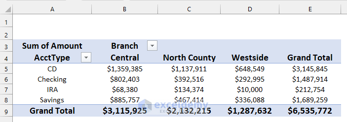
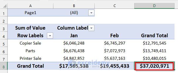
If your pivot table has the Grand Total columns for both rows and columns, you can double-click on the bottom-rightmost cell.
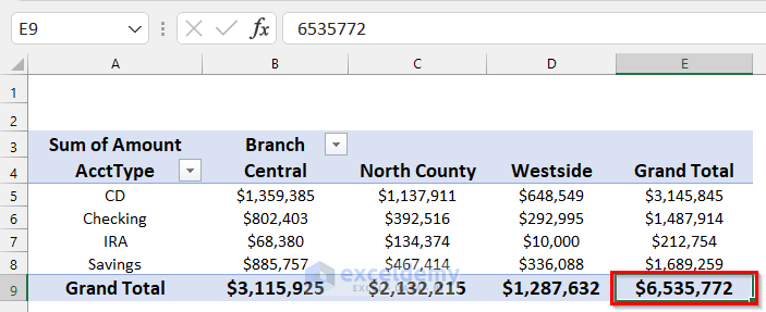
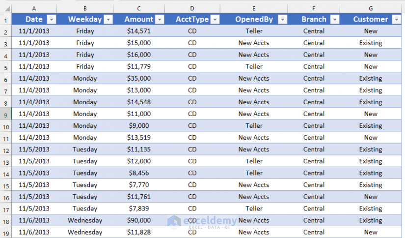
You will get the original data set of your pivot table.
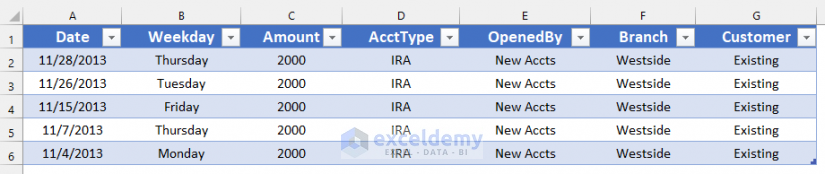
If you double-click on the cell that is the cross-section of IRA AcctType and Westside branch.
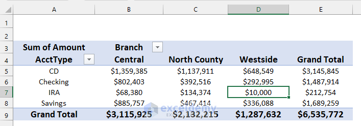
You will get the data that is related to only the IRA AcctType and Westside branch.
The original data is already stored in Pivot Cache (a kind of memory) and can be retrieved via a click.
How to Reverse a Pivot Table in Excel: 3 Easy Ways
Method 1 – Reverse a Single Range of Pivoted Data in Excel
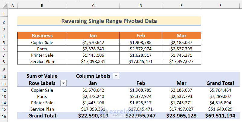
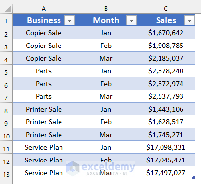
We have a data range like shown in the following image.
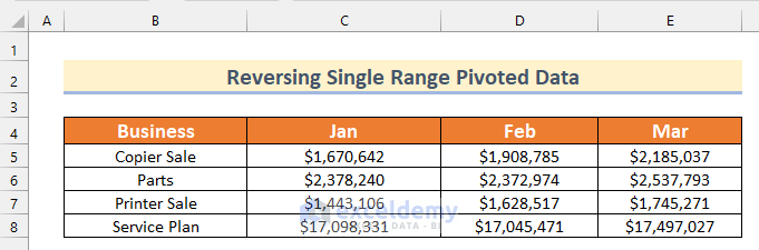
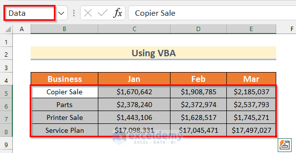
This data is showing the total sales of 4 businesses (Copier Sale, Parts, Printer Sale, and Service Plan) for the months of January to March.
When un-pivoted, this data would show under three columns (or data fields):
- Business
- Month
- Sales
For this type of data summary, we will use the PivotTable and PivotChart Wizard commands.
Step 1 – Adding the PivotTable and PivotChart Wizard to the Toolbar
- Click on the File tab.
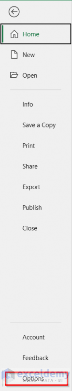
- Click on Options.
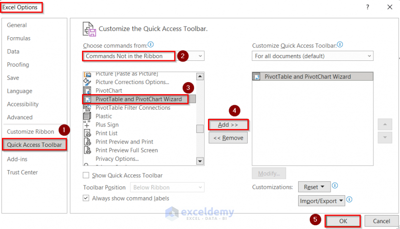
- The Excel Options box will appear.
- Go to the Quick Access Toolbar option, choose Commands Not in the Ribbon option and select PivotTable and PivotChart Wizard, then click on Add.
- Click on OK.
Step 2 – Using the PivotTable and PivotChart Wizard Command to Create Pivot Table
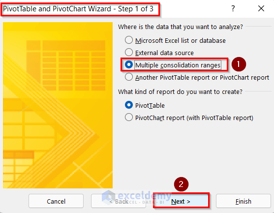
- Press the keyboard shortcut Alt + D + P to open the PivotTable and PivotChart Wizard dialog box.
- Select the Multiple consolidation ranges and PivotTable radio buttons.
- Click on the Next button.
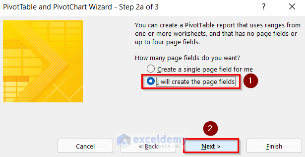
- Select I will create the page fields option and click on the Next button.
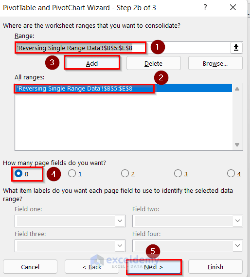
- In the Range field, select the range that you want to unpivot, then click on the Add button. The range will be inserted into the All ranges window.
- Select the range in the All ranges window; if you have just one range, then the range will be selected automatically.
- Below the All ranges window, there is an option How many page fields do you want? As we have no page fields, select 0.
- Click on OK.
- You can choose whether you will create your Excel pivot tables in a new worksheet or in the existing worksheet. We have selected the Existing worksheet option and placed the cell reference $B$10 in the field.
- Click on the Finish button.
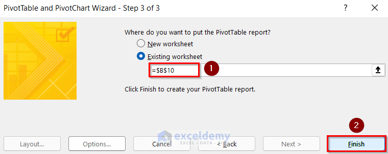
- This creates a pivot table from the given data using the PivotTable and PivotChart Wizard.
Step 3 – Reversing a Pivot Table
- Click on the bottom-right cell (cross-section of two Grand Totals) in the pivot table.
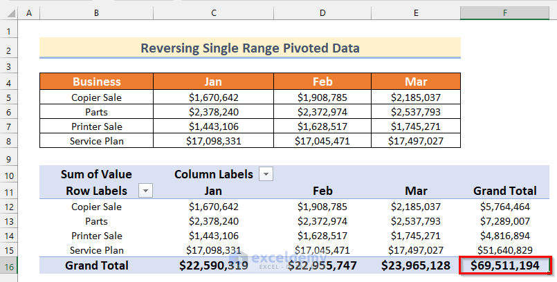
- Here is your unpivoted data.
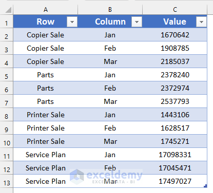
With some modifications to the table headers, your data should look like this:
Method 2 – Reverse Multiple Data Ranges in Excel
Consider the following datasets.
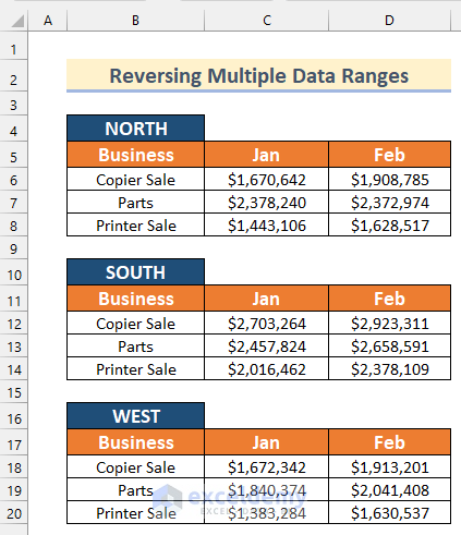
Every range has a heading: North, South, and West.
We have selected a range and then set a page field for every range.
Steps:
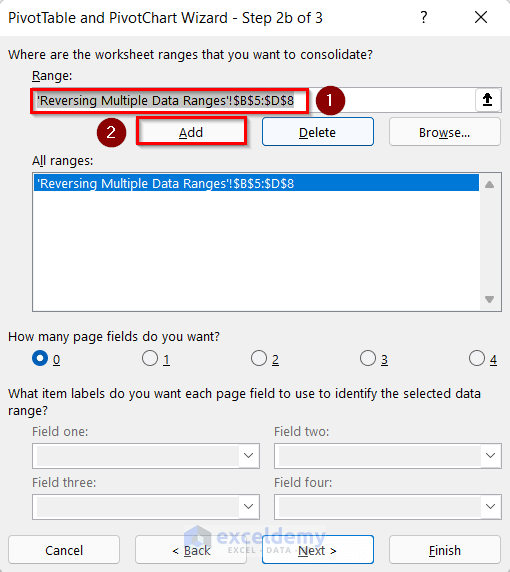
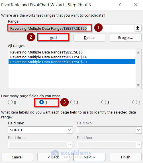
- Go through the steps shown in Method 1 to enter into Step 2b of 3 of the PivotTable and PivotChart Wizard dialog box.
- Select your first data range. We will select Cell range B5:D8 in the Range box.
- Click on the Add button.
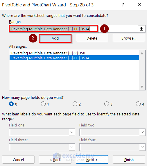
- Select your second data range. We will select Cell range B11:D14 in the Range box and click on the Add button.
- Select your third data range. We will select Cell range B17:D20 in the Range box and click on the Add button. You can have as many data ranges as you want.
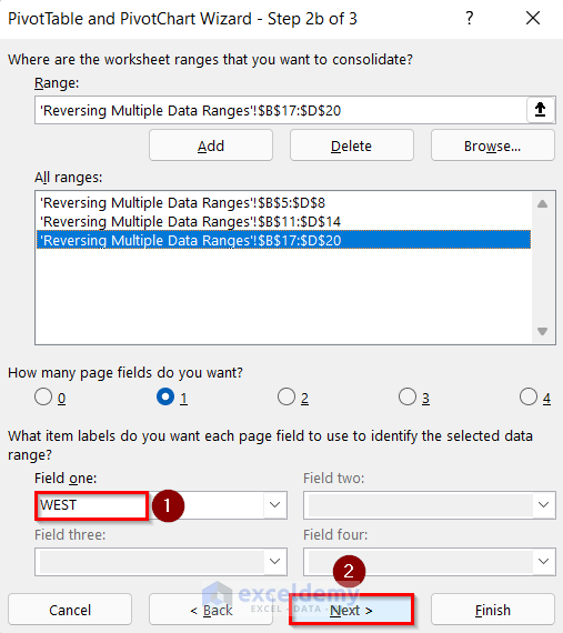
- Select 1 as the page field number.
- For the range $B$5: $D$8, we have set a page field with NORTH. For the range $B$11: $D$14, we have set the page field with SOUTH. And for the range $B$17: $D$20, we have set the page field with WEST.
- Click on Next.
- You can choose whether you will create your Excel pivot tables in a new worksheet or in the existing worksheet. We have selected New worksheet.
- Click on the Finish button.
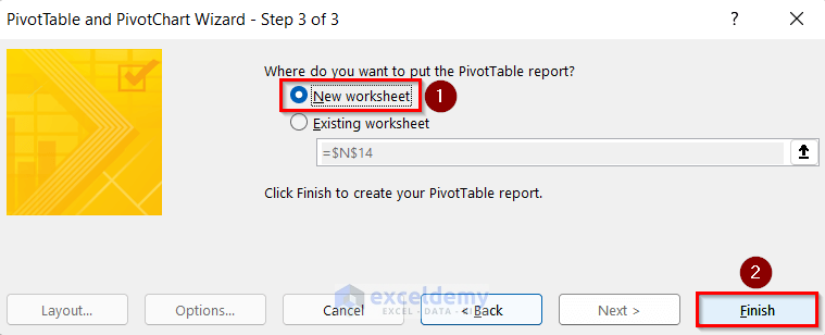
- This creates a pivot table from the given multiple data ranges using the PivotTable and PivotChart Wizard command.
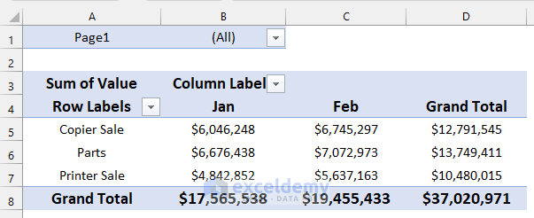
- Drill down this pivot table by clicking on the bottom-right cell (cross-section of two Grand Total) in the pivot table.
When you make an Excel Pivot Table using the PivotTable and PivotChart Wizard, four fields are created:
- Row
- Column
- Values
- And Page1 (for a single range, this field will not be created)
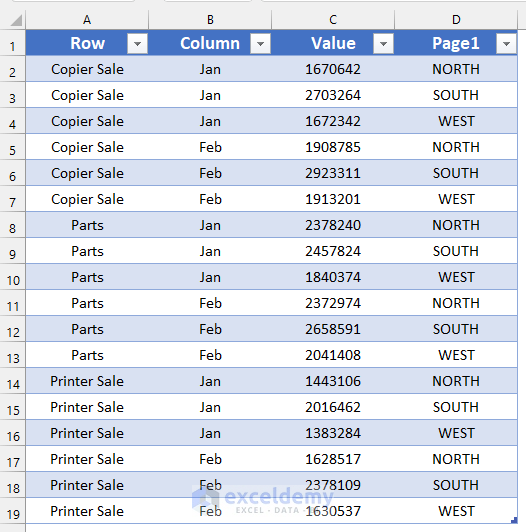
- Under the Row data field, you get the values of the first column from the data ranges. For our example, the values are Copier Sale, Parts, Printer Sale, and Service Plan.
- Under the Column data field, you will get the values of all the column headings, except the first one. The unique values in this field are Jan, Feb.
- Under the Value field, you will get all the values.
- The Page1 data field contains the original headers: NORTH, SOUTH, and WEST.
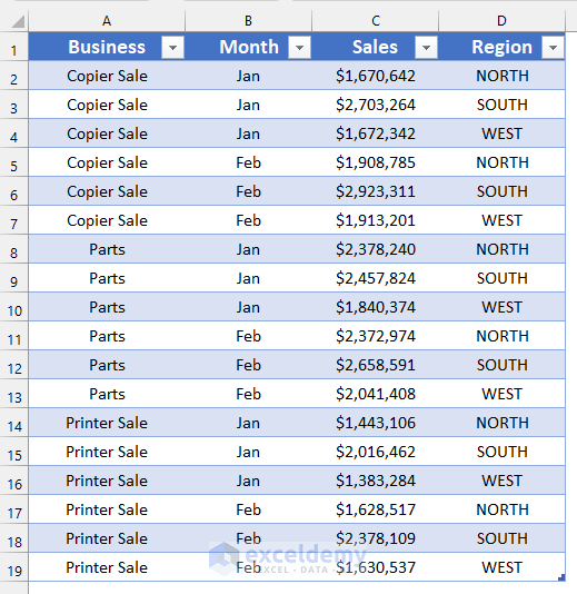
With some modifications to the table headers, your data should look like the following:
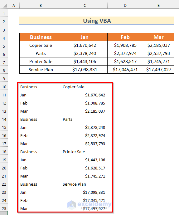
Method 3 – Using VBA to Reverse a Pivot Table in Excel
We’ll use the dataset from Method 1.
Steps:
- Name the data you want to un-pivot (without the column/row headers) using the Name Box. We will name the cell range B5:E8 as Data.
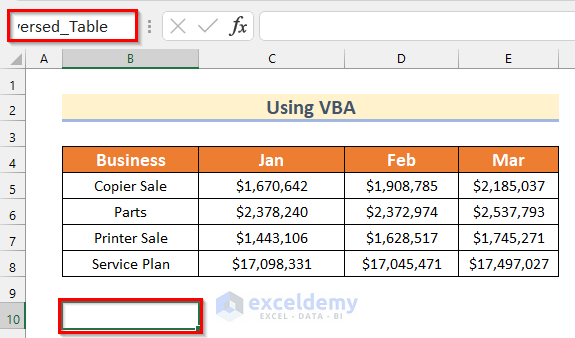
- Name the first cell using the Name Box where you want to place your output of the VBA code. We will name Cell B10 as Reversed_Table.
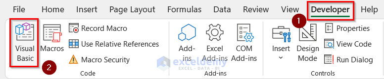
- Go to the Developer tab and click on Visual Basic.
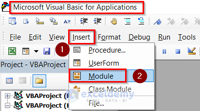
- The Microsoft Visual Basic for Application box will open.
- Click on Insert and select Module.
- Insert the following code in your Module.
Sub Reverse()
Dim Reversed_Table As Range
Dim Data As Range
Dim Cell_Value As Range
Set Data = Names("Data").RefersToRange
Set Reversed_Table = Names("Reversed_Table").RefersToRange
For Each Cell_Value In Data
    If Cell_Value.Value <> "" Then
        Reversed_Table.Activate
        Reversed_Table.Value = Cell_Value.Offset(-(Cell_Value.Row - Data.Row + 1), 0).Text
         Reversed_Table.Offset(0, 1).Value = Cell_Value.Offset(0, _
           -(Cell_Value.Column - Data.Column + 1)).Text
        Reversed_Table.Offset(0, 1).Value = Cell_Value.Text
        Set Reversed_Table = Reversed_Table.Offset(1, 0)
    End If
Next
Beep
End Sub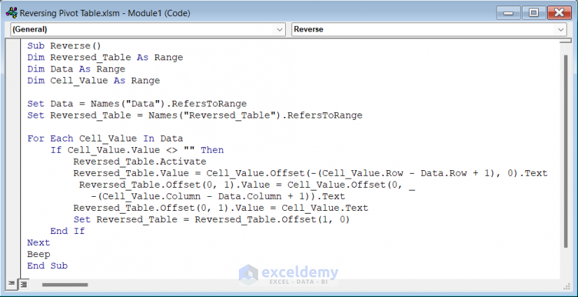
Code Breakdown
- We created a Sub Procedure as Reverse.
- We declared Reversed_Table, Data, and Cell_Value as Range.
- We set the Data equal to the value of the Named range “Data” using the RefersToRange method.
- We set the Reversed_Table equal to the value of the Named range “Reversed_Table” using the RefersToRange method.
- We used For Each loop for each Cell_Value in the Data range.
- We used the If statement to check if the value of Cell_Value is Blank, then it will activate Reversed_Table.
- In Reversed_Table stored the offset value of (Cell_Value.Row – Data.Row+1,0) using the Text method.
- We used offset(0,1) to skip 1 column from the right and then extracted text data from different rows and columns based on the Cell_Value.
- We kept all extracted Values in the Reversed_Table named range.
- Click on the Save button and go back to the worksheet.
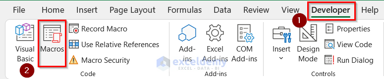
- Go to the Developer tab and click on Macros.
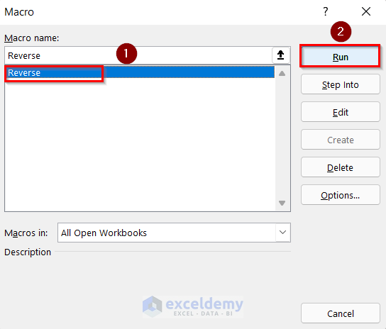
- The Macro box will appear.
- Select Reverse.
- Click on Run.
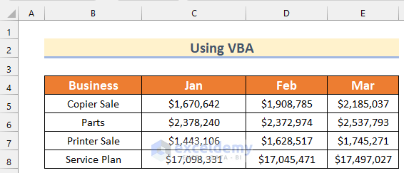
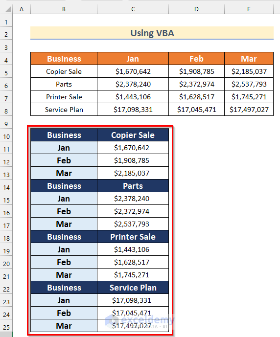
- Here is your reversed data.
You can format the data.
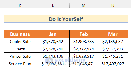
Practice Section
In this section, we are giving you the dataset to practice on your own.
Download the Practice Workbook
<<Go Back to PivotTable and Pivotchart Wizard | Pivot Table in Excel | Learn Excel
Get FREE Advanced Excel Exercises with Solutions!
