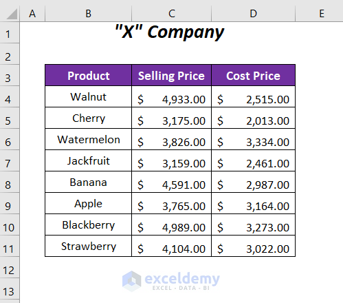
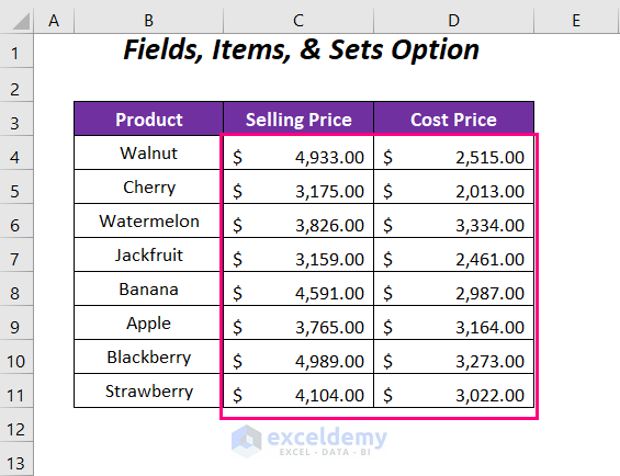
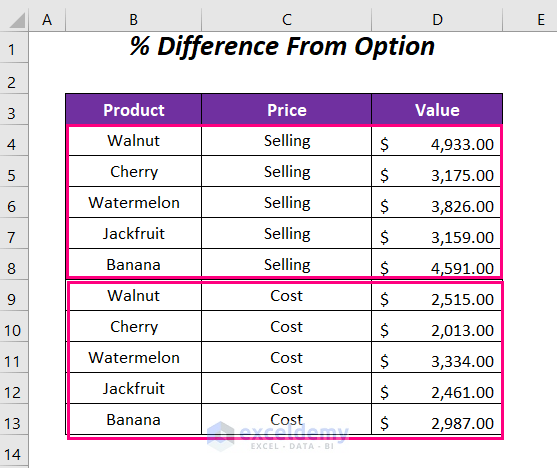
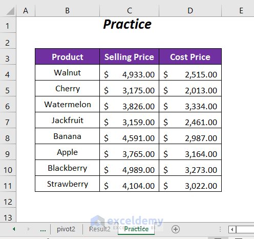
The following table contains selling and cost prices of different products.
Method 1 – Using the ‘Fields, Items, & Sets’ Option to Calculate the Percentage Difference between Two Columns in a Pivot Table
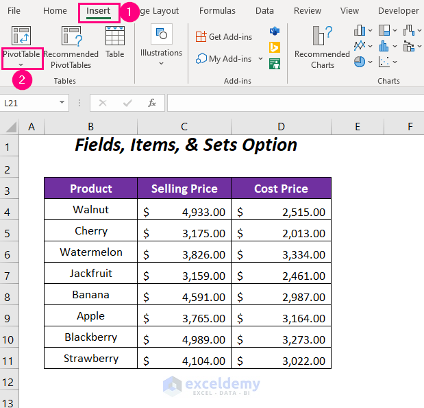
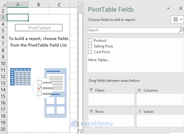
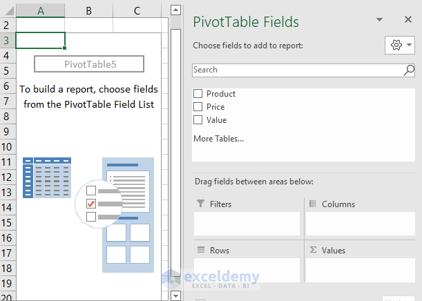
Step 1: Creating a Pivot Table
- Go to the Insert Tab >> Tables Group >>PivotTable Option.
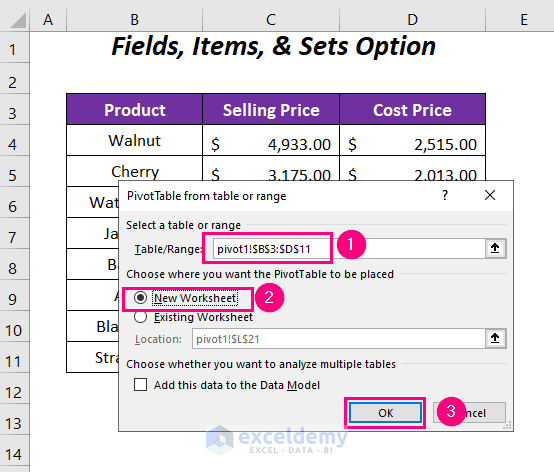
The PivotTable from table or range dialog box will be displayed.
- Select the range, click New Worksheet, and click OK.
A new sheet with PivotTable, and PivotTable Fields will be displayed.
Step 2: Calculating the Percentage Difference in the Pivot Table
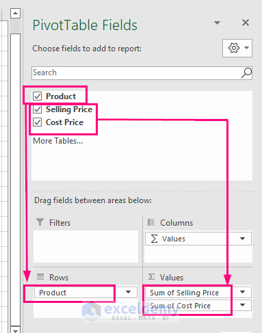
- Drag Product to Rows, Selling Price and Cost Price to Values.
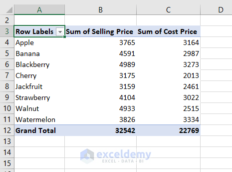
You will see the following pivot table.
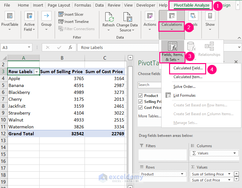
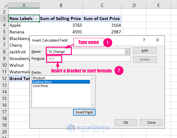
- Go to the PivotTable Analyze Tab >> Calculations >> Fields, Items, & Sets >> Calculated Field.
- Name of the new column % Change in the Name box.
- Enter =( in the Formula box.
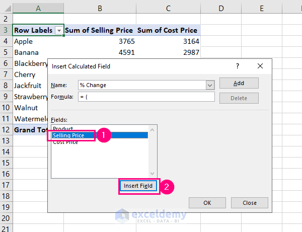
- Select the Selling Price in Fields box and click Insert Field.
The field is added to the formula.
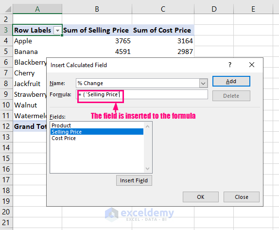
- Enter the rest of the fields into the Formula box:
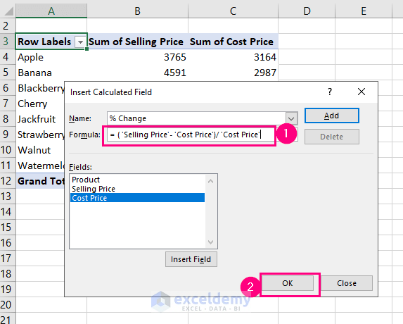
=(Selling Price-Cost Price)/Cost Price- Click OK.
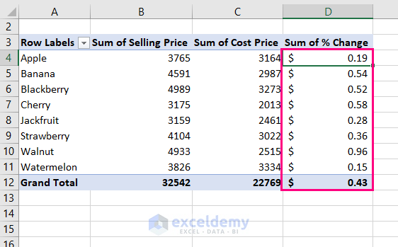
A new column with the results is displayed.
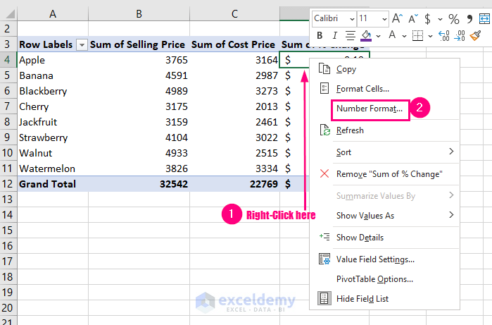
- Right-click a cell in the Sum of % Change column and select Number Format.
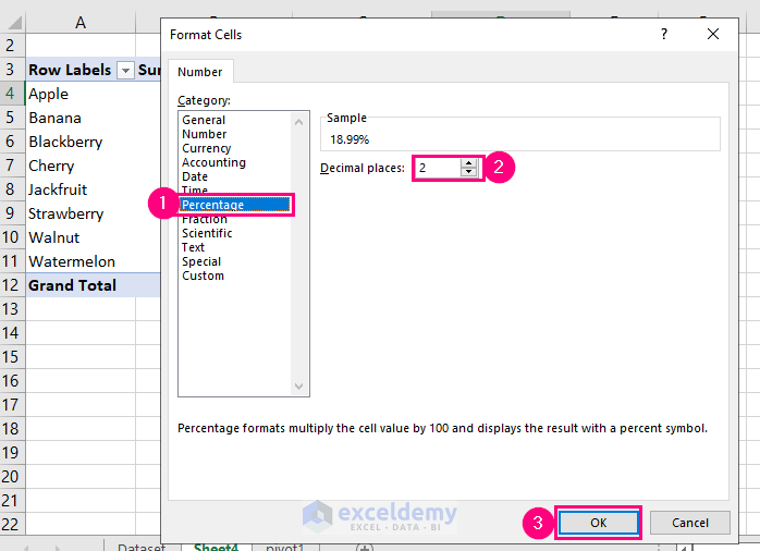
- In Format Cells, select Percentage.
- Choose the Decimal Places (here, 2).
- Click OK.
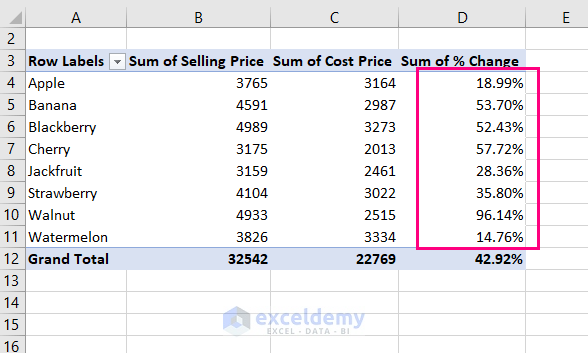
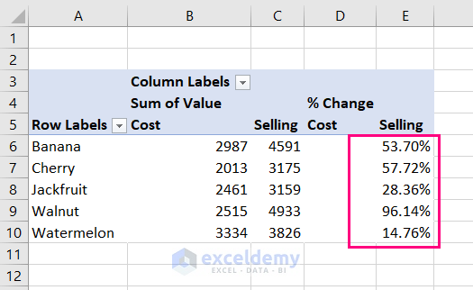
This is the output.
Read More: Excel Pivot Table: Difference between Two Columns
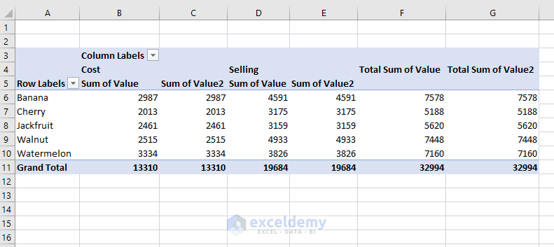
Method 2 -Using the % Difference From Option to Calculate the Percentage Difference between Two Columns
Modify the dataset like the following: combine selling and cost prices in the Value column and enter prices in the Price column.
Steps:
- Follow Step 1 in Method 1 to create the Pivot Table.
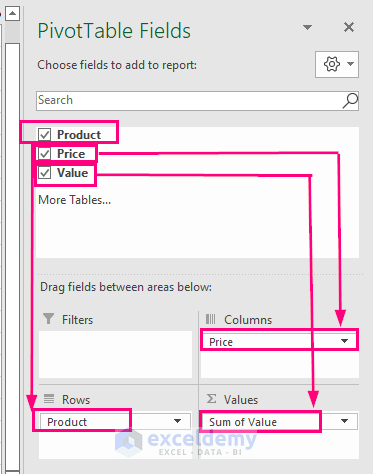
- Drag Product to Rows, Price to Columns, and Value to Values.
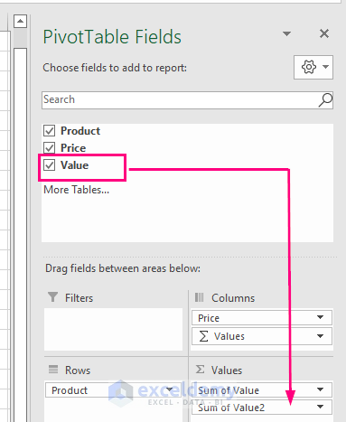
- Drag Value to Values again.
You will see the Pivot Table.
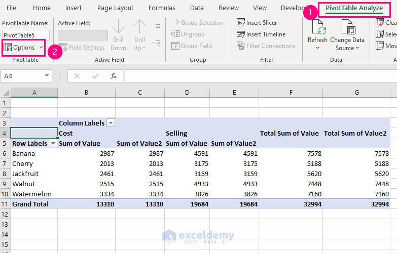
- Go to the PivotTable Analyze Tab >> PivotTable >> Options.
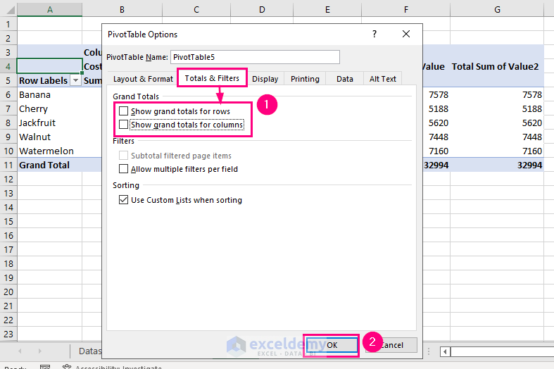
- Select Totals & Filters and uncheck the options under Grand Totals.
- Click OK.
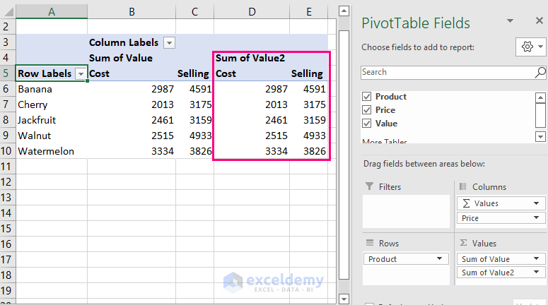
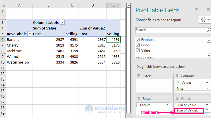
No totals are displayed, only the Sum of Value2.
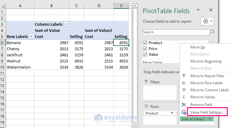
- Click Sum of Value2.
- Select Value Field Settings.
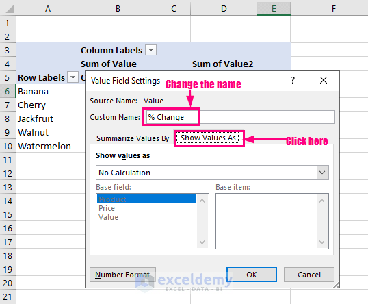
- Change the name Sum of Value2 to % Change in Custom Name.
- Click Show Values As.
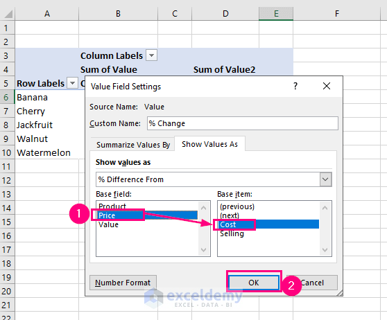
- Select Price in Base field and Cost in Base item.
- Click OK.
You will see the following percentage differences between selling and cost prices.
Practice Section
Practice here.
Read More: Calculate Difference Between Two Rows in Pivot Table
Download Workbook
<< Go Back to Pivot Table Calculations | Pivot Table in Excel | Learn Excel
Get FREE Advanced Excel Exercises with Solutions!
