Excel Pivot Table: Difference between Two Columns (3 Cases)

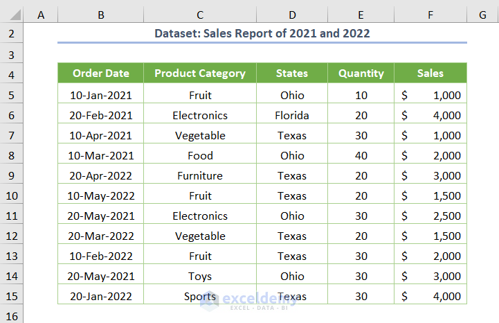
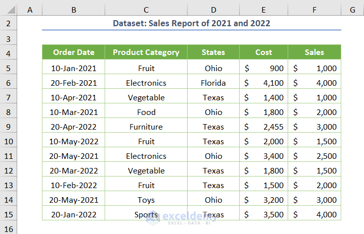
Consider the dataset which contains the Sales Report for 2021 and 2022 of some Product Categories, along with Order Date and corresponding States.

Case 1 – Utilizing the Difference from Value Field Settings Option

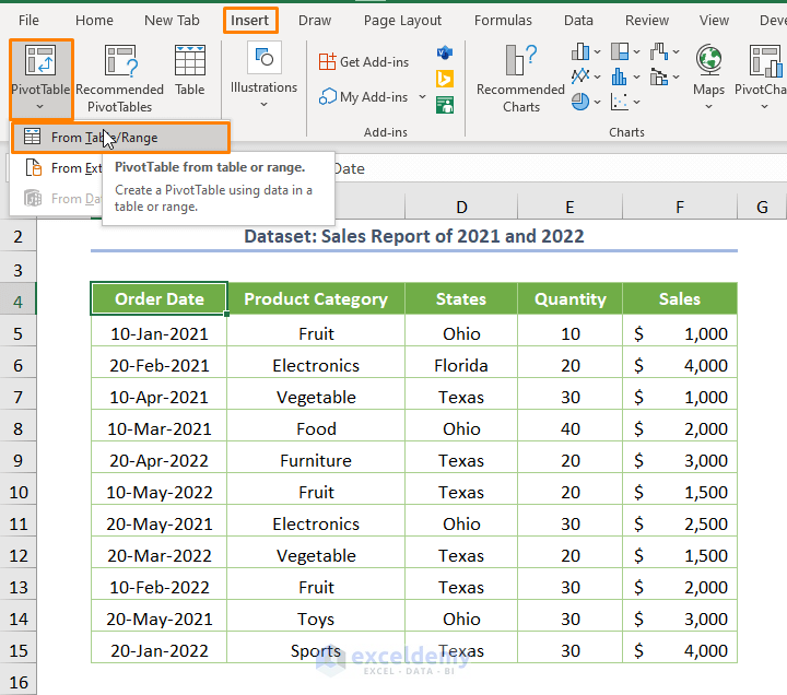
Step 1 – Create a Pivot Table

• Select any cell within the dataset.
• Go to the Insert tab, select PivotTable, and choose From Table/Range.

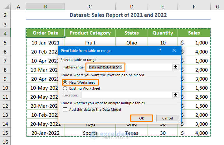
• Put the dataset in Table/Range and check New Worksheet.
• Hit OK.

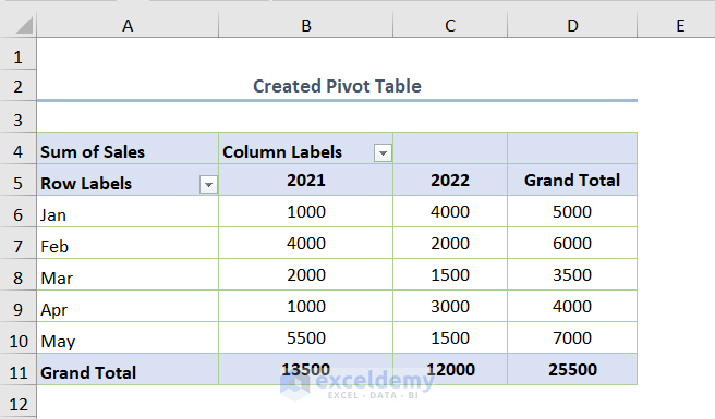
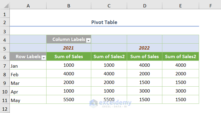
• Add (by clicking and dragging) Order Date to the Rows area, Years to the Columns area, and Sales to Values.

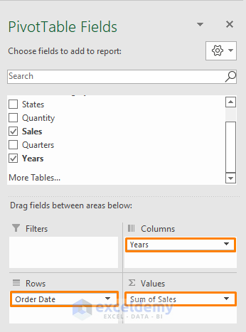
• The Pivot Table will be as follows.

Step 2 – Remove the Grand Total Column

• Go to the PivotTable Analyze tab, select Grand Totals, and choose Off for Rows and Columns.

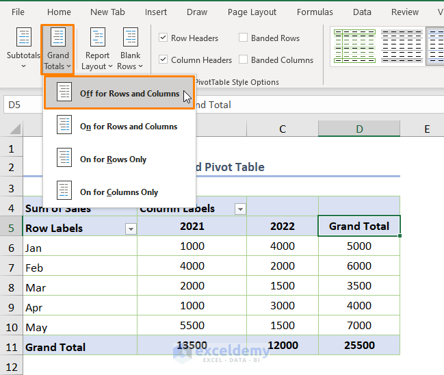
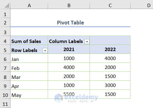
• You’ll get the following output.

Step 3 – Add the Sales Field Again

• Drag the Sales field to the Values area after the Sum of Sales.

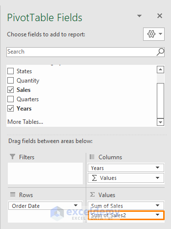
• You’ll get two similar Sum of Sales fields for a year.

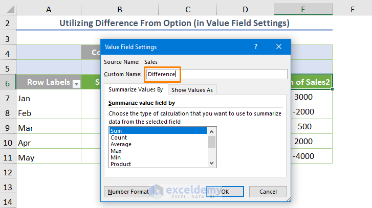
Step 4 – Apply the Difference From Option 

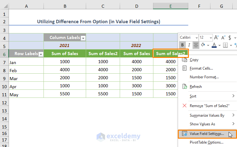
• Right-click on the Sum of Sales2 field and choose Value Field Settings.

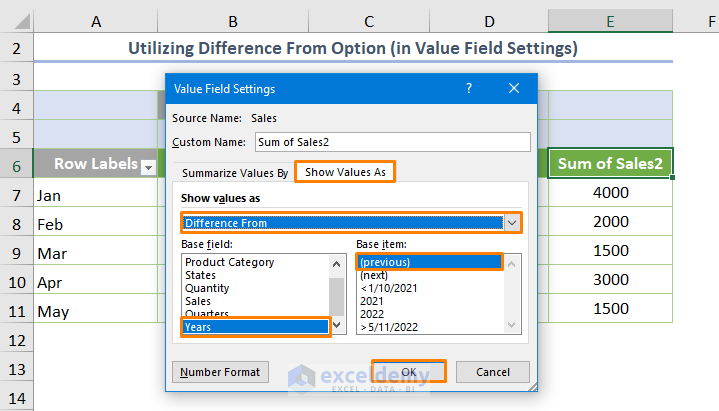
• Go to Show Values As and choose the Difference From option.
• Pick Years as the Base field and (previous) as the Base item.
• Press OK.

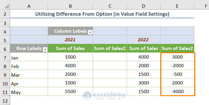
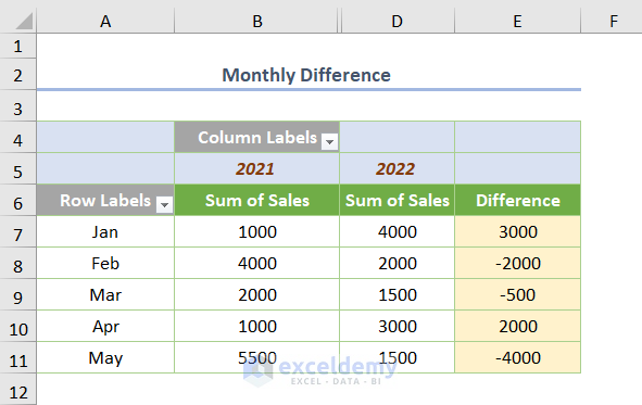
You’ll get the Difference (in the E7:E11 cells) between the Sum of Sales in 2021 and 2022.

Step 5 – Rename the Field Name and Hide Irrelevant Columns

• Double-click on the E5 cell to rename the Sum of Sales2 field to Difference.

• Hide the C column (right-click over the column and choose the Hide option).

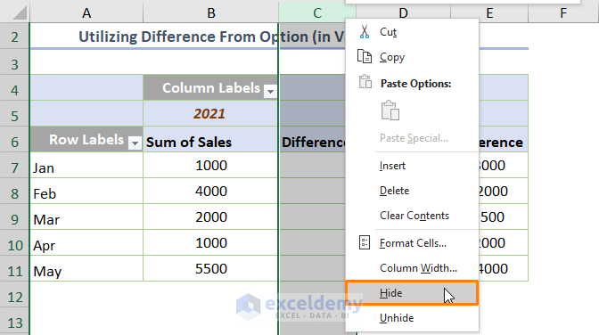
• Here’s the output.

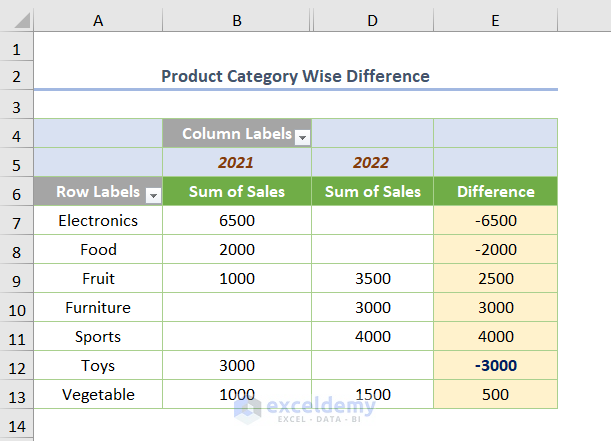
• You can also find the Difference based on the Product Category. Remove the Order Date field from the Rows area and add the Product Category field.

Read More: Calculate Difference Between Two Rows in Pivot Table

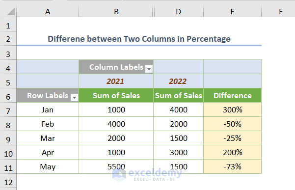
Case 2 – Showing the Difference between Two Columns in Percentages

• Repeat Steps 1-3 of Case 1 for the dataset.
• Go to the Value Field Settings and choose the % Difference From option from the Show values as.

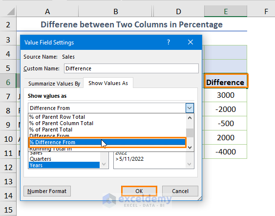
• You’ll get the Difference in % after pressing OK.

Read More: Pivot Table: Percentage Difference between Two Columns

Case 3 – Using a Formula to Show the Difference between Two Columns a Pivot Table

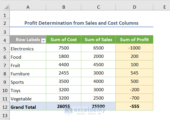
We have Cost and Sales columns in a Sales Report and need to find the Profit or Loss.

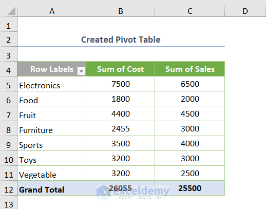
• Create a Pivot Table.

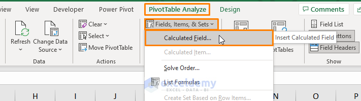
• Click the Calculated Field… option from the Fields, Items, & Sets in the PivotTable Analyze tab.

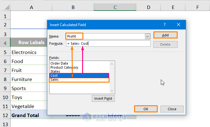
• Type the Name as Profit and insert the following formula in the Formula box.

• Double-click over the fields to add inside the formula.
• Press Add and then OK.

• You’ll get the following output.

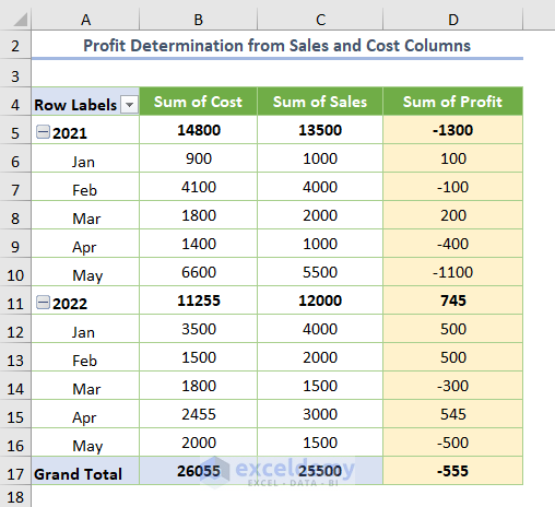
• Get the Sum of Profit yearly and monthly.

Download the Practice Workbook

<< Go Back to Pivot Table Calculations | Pivot Table in Excel | Learn Excel