How to Merge Two Pivot Tables in Excel (with Quick Steps)

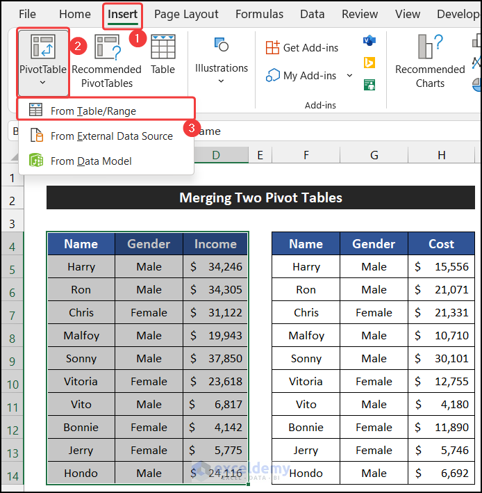
We have two Pivot Tables: Income and Cost.

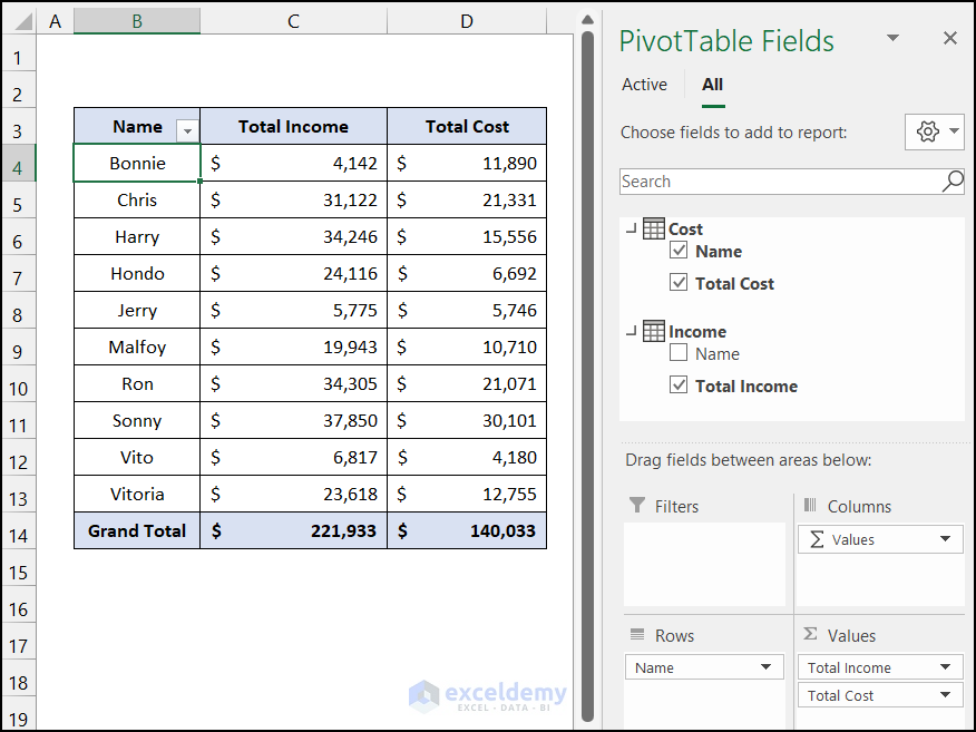
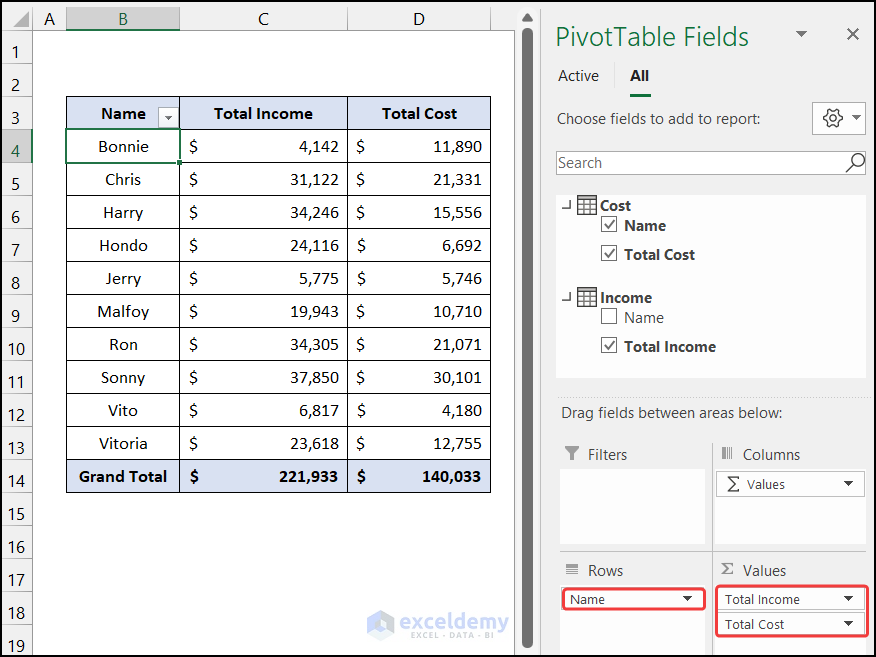
Our merged Pivot Table will look like the image shown below:

Step 1 – Create Two Different Pivot Tables

• Select the range of cells B4:D14.
• In the Insert tab, click on the drop-down arrow of the PivotTable option from the Table group and select the From Table/Range option.

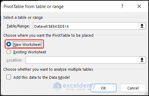
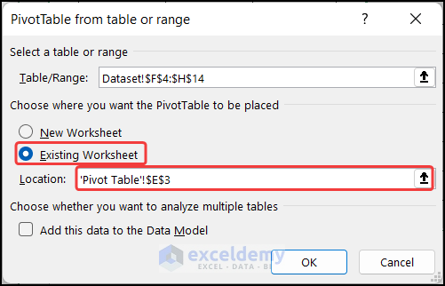
• A small dialog box called Pivot Table from table or range will appear.
• Choose the New Worksheet option.
• Click OK.

• A new worksheet will open with the Pivot Table.
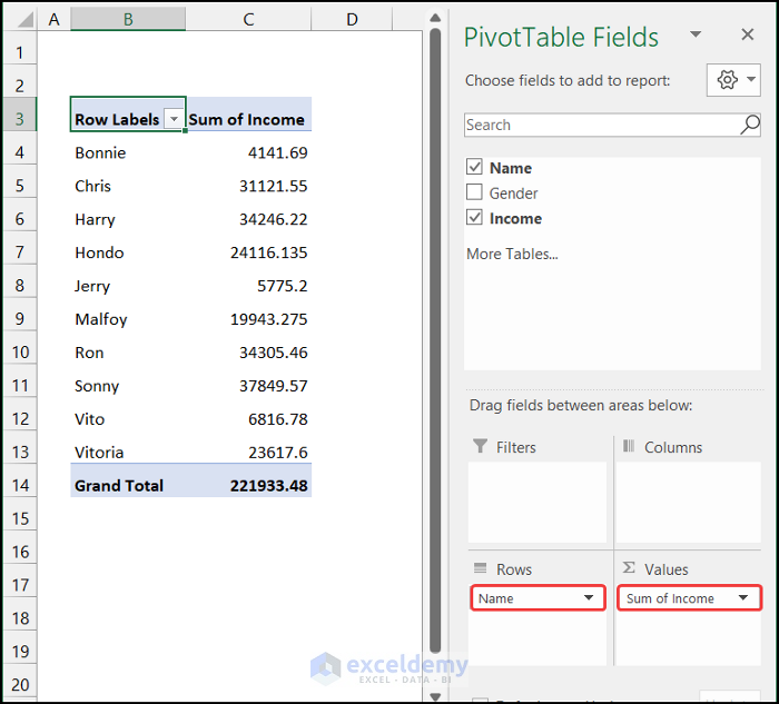
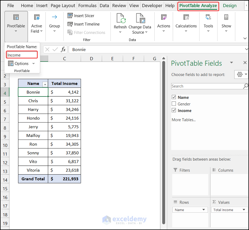
• Drag the Name field in the Rows area and the Income field in the Values area.
• The Pivot Table with data will appear.

• In the Pivot Table Analyze tab, rename the Pivot Table according in the Properties group. We set our Pivot Table name as Income.
• Format the Income Pivot Table however you want.

• Create another Pivot Table for the cost dataset. Instead of the New Worksheet option, set the destination of the Pivot Table in the Existing Worksheet and define the Location to keep both Pivot Tables in one sheet. For the second Pivot Table, we chose cell E3.

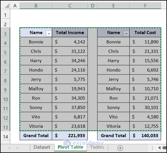
• You will get both tables on the same sheet.

Step 2 – Convert Both Pivot Tables into Conventional Tables

• Create a new sheet using the Plus (+) sign located in the Sheet Name Bar.

• Rename the sheet. We set our sheet name as Tables.
• In the Pivot Table sheet, select the range of cells B3:F13 and press Ctrl + C to copy the Pivot Tables.

• Go back to the Tables sheet.
• Right-click and paste the dataset as Values.

• You will see the dataset on that sheet.

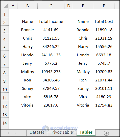
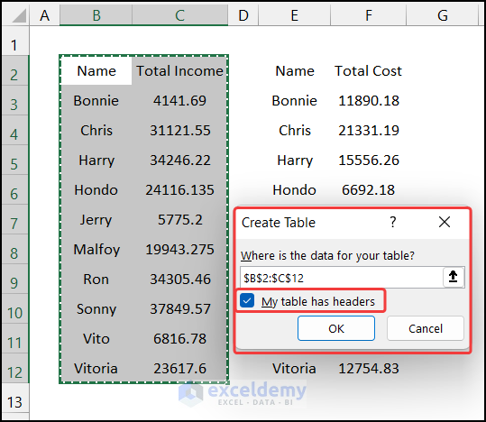
• Select the range of cells B2:C12 and press Ctrl + T to convert the data range into a table.
• A small dialog box titled Create Table will appear.
• Check the option My table has headers.
• Click OK.

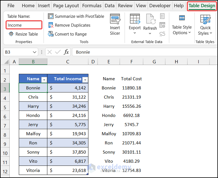
• You can rename the table in the Table Design tab, from the Properties group. We set our table name as Income.
• Format the table if you want.

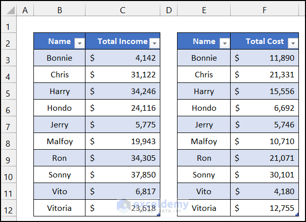
• Convert the second data range into a table as well.

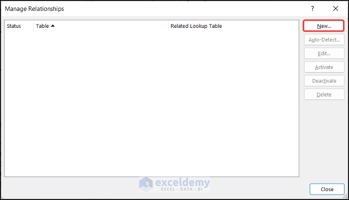
Step 3 – Establish a Relationship Between Both Tables

• Go to the Data tab.
• Select the Relationships option from the Data Tools group.

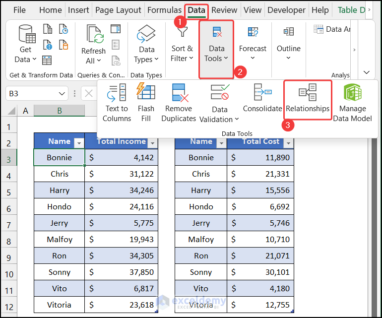
• A dialog box called Manage Relationships will appear.
• Click on the New option.

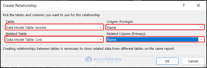
• Another dialog box titled Create Relationship will appear.
• In the Table field, select the Income table from the drop-down option, and in the Column (Foreign) field, set the Name option.
• In the Related Table field, choose the Cost table, and in the Related Column (Primary) field, select the Name option.
• Click OK.

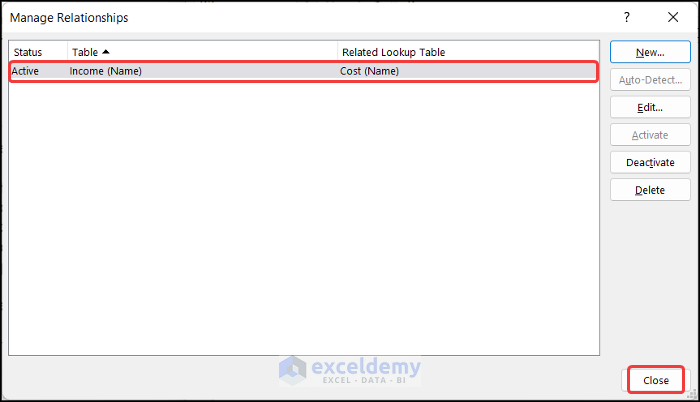
• Click the Close button to close the Manage Relationship dialog box.

Step 4 – Merge Two Pivot Tables

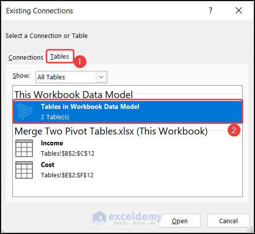
• In the Data tab, select the Existing Connections option from the Get & Transform Data.

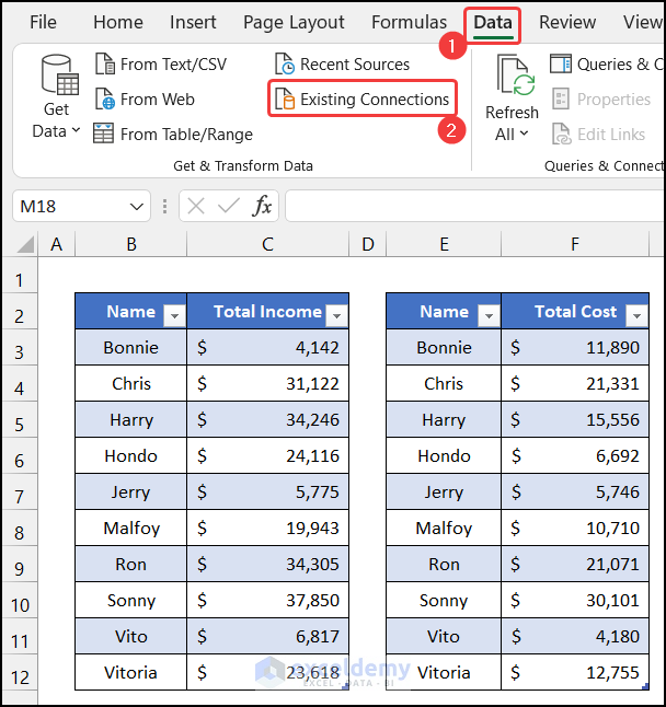
• The Existing Connections dialog box will appear.
• From the Tables tab, select the Tables in Workbook Data Model option and click on Open.

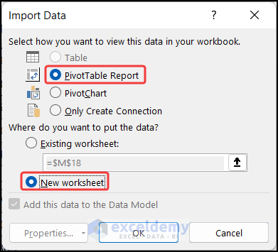
• Another dialog box titled Import Data will appear.
• Choose the Pivot Table Report option and set the destination in New Worksheet.
• Click OK.

• The Pivot Table will show in a new sheet, and both tables will show in the field list.
• Click on each table name to see the fields that belong to them.

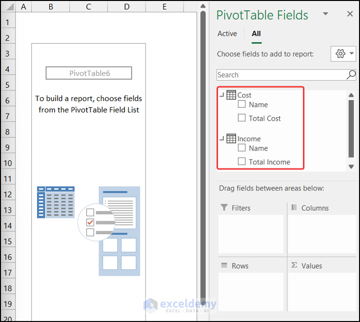
• Drag the Name field in the Rows area and the Income and Cost field in the Value area.
• You will get the final merged Pivot Table.

Download the Practice Workbook

<< Go Back to Pivot Table in Excel | Learn Excel