How to Hide Source Data in an Excel Pivot Table (With Easy Steps)

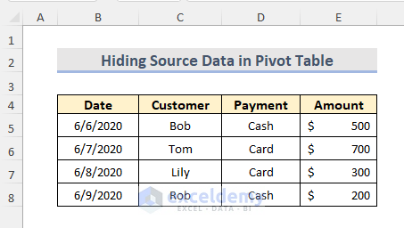
We have a dataset containing the company’s customer information about payment methods and amounts. We will create a pivot table from this dataset and hide the source data.

Step 1: Create an Excel Pivot Table

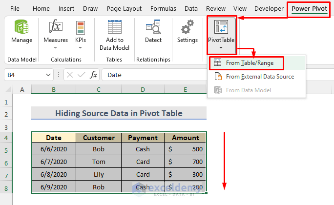
• Select the range B4:E8.
• Go to the Power Pivot tab.
• Select the PivotTable drop-down.
• Select the From Table/Range option from that drop-down.

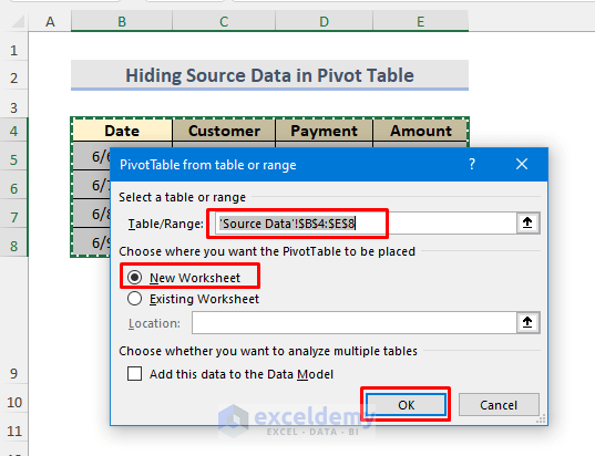
• We can see a pivot table selection window.
• In the window, select the Table/Range.
• Choose where we want to see the Pivot Table. Here, we have selected a New Worksheet.
• Press OK.

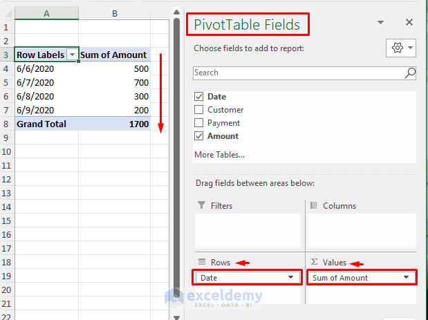
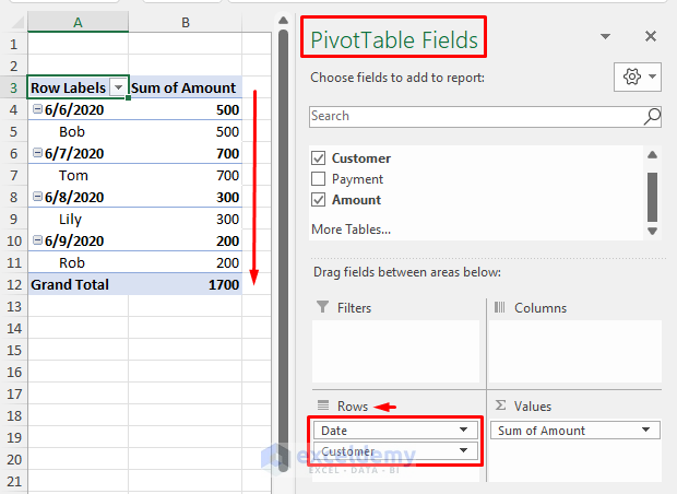
• After pressing OK, we see a PivotTable Fields list in a new worksheet (Sheet2).
• Drag the Date into the Rows area and the Amount in the Values area.
• It will create a Pivot Table in the worksheet.

Step 2: Hide Source Data in Excel

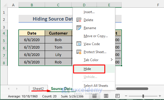
• Right-click on the sheet Source Data from the Sheet Bar.
• Select the Hide option from the context menu.
• The dataset is hidden.

Step 3: Check for Hidden Data in the Pivot Table

• Drag the Customer option in the Rows area; we can see the hidden information still shows.

• Select cell B4 in Sheet2 and double-click on it.

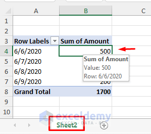
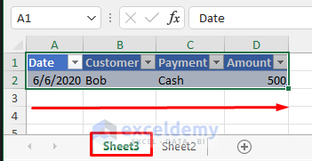
• It will create a new worksheet (Sheet3) with hidden information.

Step 4: Apply Excel PivotTable Options

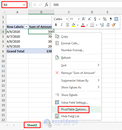
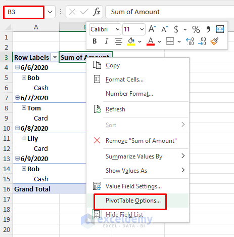
• Select cell B4 at first.
• Right-click on it.
• From the Context Menu, select PivotTable Options.

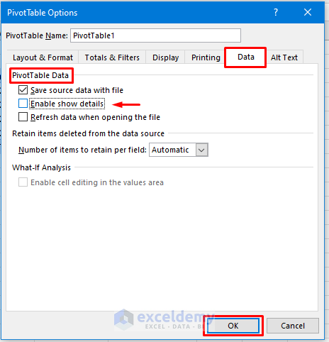
• This will take us to the PivotTable Options window.
• Go to the Data tab.
• From PivotTable Data, uncheck the Enable Show Details option.
• Press OK.

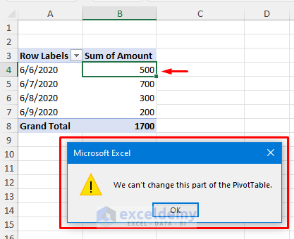
Final Output

In the pivot table, if we double click on any cell, it’ll show us a message ‘We can’t change this part of the PivorTable’ (See Screenshot). That means we successfully hide the source data in the Excel Pivot Table.

How to Hide a Pivot Table Field List in Excel

STEPS:

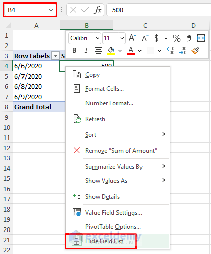
• Select cell B4 of the pivot table.
• Right-click on it to see the context menu.
• Select the Hide Field List option.
• The field list is hidden and it only appears when we click on the pivot table data.

• Use Excel VBA to hide this field list.
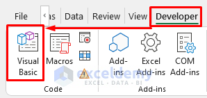
• Go to the Developer tab.
• Select the Visual Basic option.

• This will open a Visual Basic Editor window.
• Go to the Insert tab.
• Select the Module option.

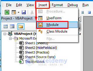
• A VBA Module window opens here. We can open it using the keyboard shortcut ‘Alt + F11’.
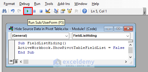
• Enter the following code:

Sub FieldListHiding()
ActiveWorkbook.ShowPivotTableFieldList = False
End Sub

• Click on the Run option, or press the F5 key to run the code.

• A confirmation Macros window pops up.
• Select the sheet name and click on the Run.

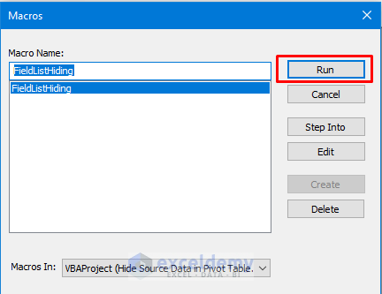
• It will hide the pivot table field list.

Sub FieldListHiding()
ActiveWorkbook.ShowPivotTableFieldList = True
End Sub

How to Hide a Pivot Table Data in Excel

STEPS:

• Select the required data that we want to delete.

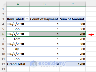
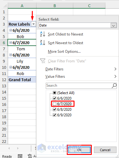
• Select the arrow in the Row Labels cell.
• Uncheck the value that we don’t want to see.
• Click on OK.

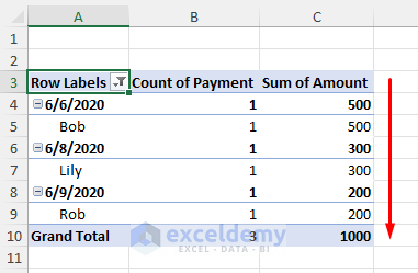
• The data is hidden in the pivot table.

How to Protect Source Data from Being Hidden in Excel

STEPS:

• Right-click on any cell of the pivot table.
• Select PivotTable Options.

• This will take us to the PivotTable Options window.
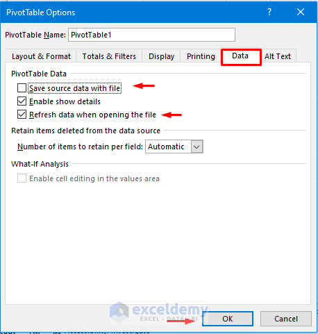
• Go to the Data tab.
• Uncheck the option Save source data with file.
• Check the option Refresh data when opening the file.
• Click OK.

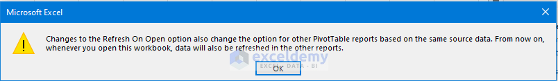
• This will protect the source data from being hidden and show us the below message box.

• If we don’t checkmark the option Refresh data when opening the file, we will see the message below.

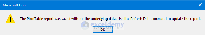
• To avoid that, we will need to refresh data manually after filtering data, which is very irritating. So it’s better to put a checkmark on that option.

Download the Practice Workbook

Download the following workbook to practice.

Related Articles

• Pivot Table is Not Picking up Data in Excel
• Excel VBA to Change Pivot Table Source

<< Go Back to Pivot Table Data Source | Pivot Table in Excel | Learn Excel