How to Add Hyperlink to Cell Value in Excel Using VBA (4 Methods)

Method 1 – Embed VBA to Add Hyperlink from a Different Worksheet to a Cell Value in the Active Sheet

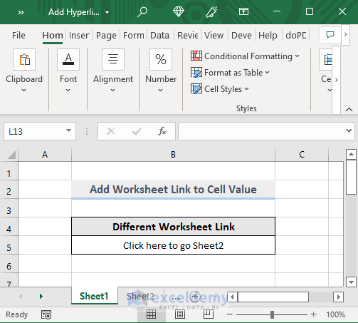
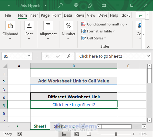
Let’s consider the following dataset: In our workbook, we have the value “Click here to go to Sheet2” in Cell B5 of Sheet1. We’ll learn how to use VBA code to add a link to Sheet2 within the cell value of B5 in Sheet1.

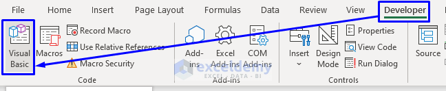
First, press Alt + F11 on your keyboard or go to the Developer tab and select Visual Basic to open the Visual Basic Editor.

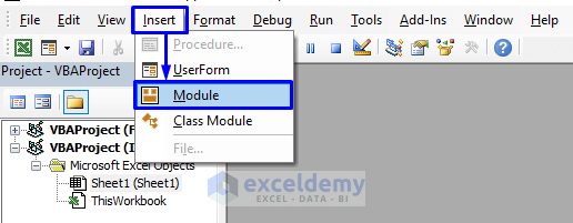
In the code window that pops up, click Insert > Module from the menu bar.

Copy the following code and paste it into the code window:

Sub HyperlinkAnotherSheet()
Worksheets("Sheet1").Select
Range("B5").Select
ActiveCell.Hyperlinks.Add Anchor:=Selection, Address:="", SubAddress:="'Sheet2'!A1"
End Sub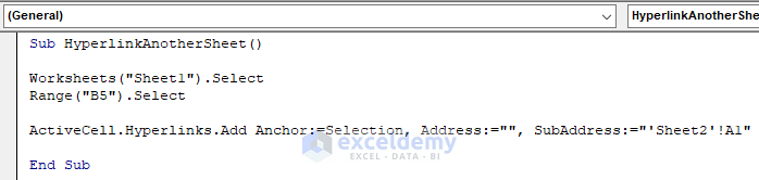

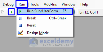
Your code is now ready to run. Press F5 on your keyboard or select Run > Run Sub/UserForm from the menu bar. Alternatively, click the small Run icon in the sub-menu bar to execute the macro.

After successful execution, the cell value of B5 in Sheet1 will be linked to worksheet Sheet2. To verify whether the link works, click on the link.

VBA Code Explanation

Sub HyperlinkAnotherSheet()

To name the sub-procedure of the macro.

Worksheets("Sheet1").Select

Selects the worksheet containing the cell whose value will be linked.

Range("B5").Select

Specifies the cell whose value will be linked.

ActiveCell.Hyperlinks.Add Anchor:=Selection, Address:="", SubAddress:="'Sheet2'!A1"

Defines the destination. Cell A1 of Sheet2 will be opened after clicking the cell value (B5).

End Sub

To leave the sub-procedure of the macro.

Method 2 – Apply Macro to Add Hyperlink from Multiple Worksheets to Multiple Cell Values in Active Sheet

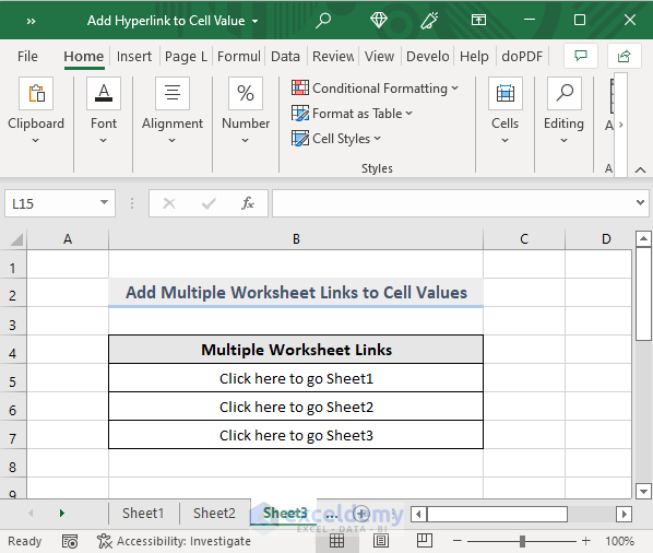
In this section, we’ll learn how to hyperlink multiple worksheets to various cell values in the active worksheet using VBA. Let’s look at the dataset above. We want to link values in Cells B5, B6, and B7 of worksheet Sheet3 to worksheets Sheet1, Sheet2, and Sheet3, respectively.

Open the Visual Basic Editor from the Developer tab and insert a new module in the code window.
Copy the following code and paste it into the module:

Sub HyperlinkMultipleSheets()
Dim iSheet As Worksheet
Worksheets("Sheet3").Select
Range("B5").Select
For Each iSheet In ActiveWorkbook.Worksheets
    ActiveCell.Hyperlinks.Add Anchor:=ActiveCell, Address:="", SubAddress:="" & iSheet.Name & "!A1" & "", ScreenTip:=""
    ActiveCell.Offset(1, 0).Select
Next iSheet
End Sub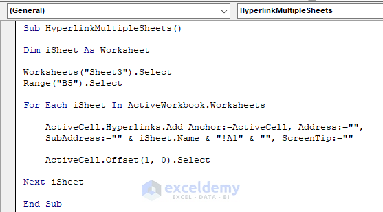

Your code is now ready to run. Execute the macro as shown in the previous section. The result is displayed in the image below:

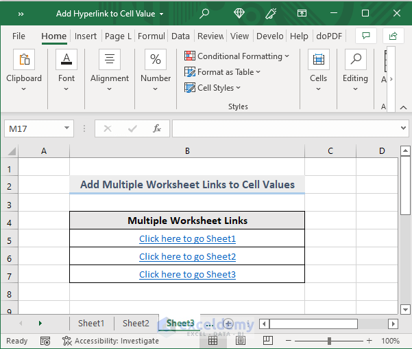
To verify whether the links work, click on the links created in Cells B5, B6, and B7 of worksheet Sheet3. Each link will take you to the corresponding worksheets (Sheet1, Sheet2, and Sheet3).

VBA Code Explanation

Sub HyperlinkMultipleSheets()

To name the sub-procedure of the macro.

Dim iSheet As Worksheet

Declares the variable to store the worksheet.

Worksheets("Sheet3").Select

Selects the worksheet containing the cell whose value will be linked.

Range("B5").Select

Specifies the cell whose value will be linked.

For Each iSheet In ActiveWorkbook.Worksheets
    ActiveCell.Hyperlinks.Add Anchor:=ActiveCell, Address:="", SubAddress:="" & iSheet.Name & "!A1" & "", ScreenTip:=""
    ActiveCell.Offset(1, 0).Select
Next iSheet

Iterating through all worksheets in the active workbook. It will go through each row and link them with the worksheets, starting from the very first sheet to the last one by setting the destination to Cell A1 of every worksheet. It continues to do this till it finishes iterating through every sheet in the active workbook.

End Sub

To leave the sub-procedure of the macro.

Method 3 – Implement VBA to Insert Value in Cell and Add Hyperlink Automatically in Excel

Wouldn’t it be interesting if you could automatically insert hyperlinks into cell values when you add specific words? Let’s explore how to achieve this using a VBA macro in Excel.

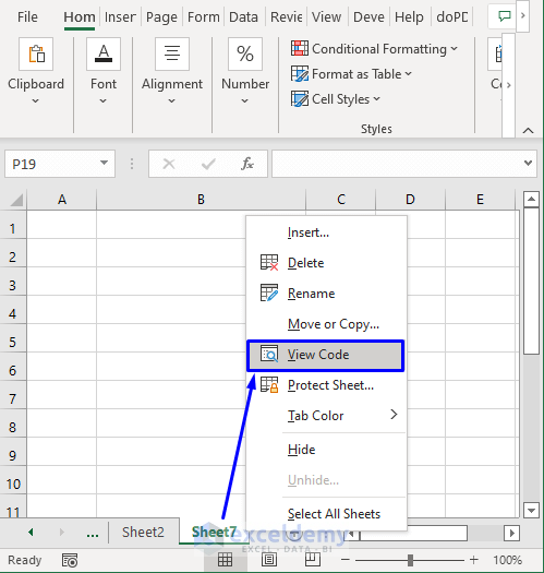
Open your Excel workbook and navigate to Sheet7.
Right-click on the sheet and select View Code from the list of options.

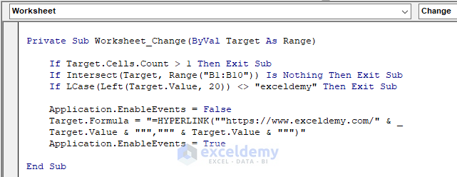
Insert the following code directly into the code window under the specified sheet (not in any module):

Private Sub Worksheet_Change(ByVal Target As Range)
    If Target.Cells.Count > 1 Then Exit Sub
    If Intersect(Target, Range("B1:B10")) Is Nothing Then Exit Sub
    If LCase(Left(Target.Value, 20)) <> "exceldemy" Then Exit Sub
    Application.EnableEvents = False
    Target.Formula = "=HYPERLINK(""https://www.exceldemy.com/" & Target.Value & """,""" & Target.Value & """)"
    Application.EnableEvents = True
End Sub

Don’t run this code, save it.

If you look at the code, you will see:

In the 3rd line of the macro, we declare range B1:B10.
In the 4th line of the code, we wrote the word “exceldemy”.
We provided the link to the ExcelDemy website one line later.

This whole process means that every time you enter the word “exceldemy” in the range B1:B10 of your dataset, the word “exceldemy” will be automatically linked to the ExcelDemy website.

VBA Code Explanation

If Target.Cells.Count > 1 Then Exit Sub
If Intersect(Target, Range("B1:B10")) Is Nothing Then Exit Sub
If LCase(Left(Target.Value, 20)) <> "exceldemy" Then Exit Sub

This piece of code specifies the range B1:B10 for inserting the word “exceldemy“.

Application.EnableEvents = False

To turn off any kind of events to take place while the code is running.

Target.Formula = "=HYPERLINK(""https://www.exceldemy.com/" & Target.Value & """,""" & Target.Value & """)"

Every time you enter the specified word (“exceldemy“) in no other range than B1:B10, then it will be linked with the address of “https://www.exceldemy.com/“.

Application.EnableEvents = True

Turning back on the EnableEvents property of the application.

Method 4 – Embedding a VBA Macro to Add Hyperlink to Cell Values by Selection in Excel

In this method, we’ll explore how to link a specific cell value to a website (in this case, the ExcelDemy website) by selecting the cell after executing a VBA code. Let’s walk through the steps:

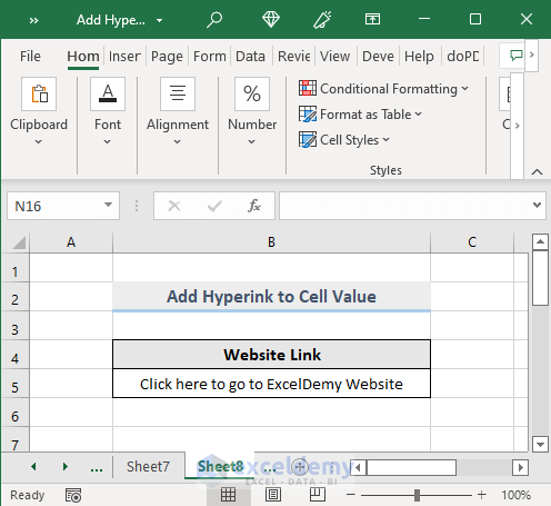
Open your Excel workbook and locate Sheet8.
Open Visual Basic Editor from the Developer tab and Insert a Module in the code window.
Copy the following code and paste it into the code window:

Option Explicit
Sub HyperlinkWebsite()
Dim iRange As Range
On Error Resume Next
Set iRange = Application.Selection
Set iRange = Application.InputBox("Select Range to Add Link", "Range", iRange.Address, Type:=8)
Dim i As Long
Dim iLink As String
For i = iRange.Rows.Count To 1 Step -1
  If iRange.Cells(i, 1).Value <> "" Then
    iLink = "https://www.exceldemy.com/" & CStr(iRange.Cells(i, 1).Value)
      iRange.Cells(i, 1).Hyperlinks.Add Anchor:=iRange.Cells(i, 1), Address:=iLink, TextToDisplay:=CStr(iRange.Cells(i, 1).Value)
   End If
  Next
End Sub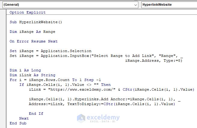

Run the code.
In the pop-up window, select Cell B5.
Press OK.

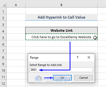
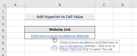
Cell B5 will be linked to the link that you provided in the code.

VBA Code Explanation

Option Explicit

In the beginning, the code forces explicit declaration of all variables in the file.

Sub HyperlinkWebsite()

Then, names the sub-procedure of the macro.

Dim iRange As Range

After that, declares the variable to hold the selected range.

On Error Resume Next

If any error occurs, then go to the next statement.

Set iRange = Application.Selection
Set iRange = Application.InputBox("Select Range to Add Link", "Range", iRange.Address, Type:=8)

Defines the selection operation from the user input.

Dim i As Long
Dim iLink As String

Declaring the variables to perform loop operation.

For i = iRange.Rows.Count To 1 Step -1

Starts looping from the last row count to the first row.

If iRange.Cells(i, 1).Value <> "" Then
  iLink = "https://www.exceldemy.com/" & CStr(iRange.Cells(i, 1).Value)
  iRange.Cells(i, 1).Hyperlinks.Add Anchor:=iRange.Cells(i, 1), Address:=iLink, TextToDisplay:=CStr(iRange.Cells(i, 1).Value)

To link the selected cell with the link address of “https://www.exceldemy.com/“.

End If

End of IF statement.

Next

End of FOR loop.

End Sub

How to Add Hyperlink to Cell Value in Excel Using VBA (4 Methods)

Method 1 – Embed VBA to Add Hyperlink from a Different Worksheet to a Cell Value in the Active Sheet

Method 2 – Apply Macro to Add Hyperlink from Multiple Worksheets to Multiple Cell Values in Active Sheet

Method 3 – Implement VBA to Insert Value in Cell and Add Hyperlink Automatically in Excel

Method 4 – Embedding a VBA Macro to Add Hyperlink to Cell Values by Selection in Excel

Leave a reply Cancel reply